


 Inglés (pdf)
 Articulo en XML
 Referencias del artículo
 Enviar articulo por email
 Citado por SciELO
  Similares en
SciELO
Similares en
SciELO 
 Permalink
Introduction
According to Federcitrus (2022), citrus production in Argentina amounts to approximately 3.5 million tons, with sweet oranges roughly contributing 1 million tons and Valencia late being the most important variety. The cultivation area for Salustiana is increasing, and mandarins contribute around 500,000 tons, with Tangor Murcott as one major type.
Estimating citrus yield is challenging due to interannual and individual variations in productive traits. Typically, estimation relies on agronomic conditions, tree characteristics, historical orchard yield, and subjective observations, leading to estimation errors ranging from 15% to 25% ( Apolo-Apolo et al., 2020 ). Recently, precision agriculture incorporating computing, robotics, artificial intelligence, and remote sensing, has improved yield estimation accuracy.
Several researchers have explored remote sensing and machine learning methods to predict crop yield. Córdoba et al. (2012) employed PCA (principal component analysis) to assess spatial covariation of soil properties and crop yield. Teixidó et al. (2018) developed semi-automated methods using different image capture systems and segmentation techniques. Wang et al. (2021) successfully tested various image capture methods by developing target image detection technology for remote sensing images based on deep learning.
Remote sensing data captured by civilian satellite-borne sensors enables monitoring Earth surface at different temporal and spatial scales. Begué et al. (2018) highlighted the convenience of using these images, which offer low costs per unit area while providing consistent spatial and temporal comparisons of vegetation conditions. Various vegetation indices have been developed, including the Standard Vegetation Difference Index (NDVI) for monitoring vegetation biomass. Arango et al. (2016a , 2016b, 2017) employed MODIS sensor images and associated variables such as soil properties, biophysical characteristics of crop sites, cultural treatments, and production, identifying arable land.
Machine learning techniques, including support vector machines (SVM), random forest (RF), and artificial neural networks (ANN), have proven effective in estimating agricultural variables of interest. Díaz et al. (2017) and Bóbeda et al. (2018) used machine learning systems to predict citrus production and load, respectively. Taghizadeh et al. (2020) employed SVM and RF algorithms to forecast land suitability for rain-fed wheat and barley. Numerous studies have explored the use of machine learning algorithms to predict crop yield for maize, and potato tuber, among other crops.
The objectives of this study are to identify low-cost and accessible variables for estimating citrus harvest while developing a methodology for early estimation of fruit number per tree using remote sensing and machine learning techniques.
Material and Methods
Area and Material of Study
The study collected empirical data from citrus-producing orchards located in the Corrientes and Entre Rios provinces, northeastern Argentina, with geographical coordinates 27°39´39” to 31°23´59” S and 57°00´01” to 58°58´59” W. Orchard age ranged from 7 to 30 years and varietal composition included 44% Murcott tangor ( Citrus reticulata x C. sinensis), 52% Valencia late, and 4% Salustiana sweet oranges ( C. sinensis). Among the orchards, only 40% were irrigated, 78% of the trees were planted in sandy soil, and 22% were planted in clayey soil. Salustiana orchards were included in the dataset to increase variability, but further research is needed to develop a yield estimation model for this variety.
The dataset comprised three types of variables: tree and orchard characteristics, climatic variables, and satellite information. Field data were collected using a systematic random sampling method during the 2005/06 to 2015/16 seasons. The sample included 2-3% of trees from each orchard, and the following information was gathered:
Harvest: The target variable is the average count of fruits per tree recorded during harvest in each orchard.
Orchard characteristics: This category includes species (tangerine, sweet orange); variety (Murcott, Salustiana, Valencia late); soil type (sandy, clayey); irrigation (presence, absence); and age.
Tree traits: Canopy height and trunk diameter in meters. To estimate harvest time, fruits were counted in a sampling frame of 0.125 cubic meters at 1.5 meters from the ground and at the four cardinal points of the canopy. Then, fruits were manually counted 60 and 30 days before the estimated harvest time. Average number of fruits was calculated.
Climatic variables: This category included total rainfall, average temperature, and humidity during full bloom (September), fruit growth (December to March), and ripening (April to July). These data were obtained from weather stations located 5 to 45 km from the orchards.
Satellite information: MODIS data were used to obtain near-infrared reflectance, red reflectance, and NDVI during full bloom (September), fruit growth and ripening (December to June). Two monthly records allowed average value calculations for each month. NDVI is defined as
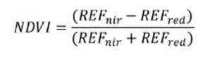
where REFnir is Reflectance in the infrared spectrum and REFred, in the red spectrum.
MODIS is aboard the Terra and Aqua satellites. The primary product used in this study was MOD091, which provides reflectance data for terrestrial coverage assessment with daily temporal resolution and a spatial resolution of 250 m. NDVI and reflectance values, as well as database organization related to orchards, followed an automated extraction process outlined in a four-stage workflow depicted in Figure 1 (a) (page 68): (1) Orchards location, and centroids calculation.
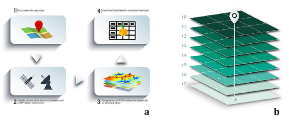
Figure 1(a): Steps for data extraction from MODIS sensor. Figure 1(b): Maps t-layer containing monthly NDVI summary for each moment (0 to t7). Figura 1(a): Etapas del proceso de extracción data del sensor MODIS. Figura 1(b): t-capas de mapas con los resúmenes mensuales de NDVI por momento (0 a 7).
(2) The MODIS sensor time series product MOD09GQ1 download using R Statistics routine ( Arango et al., 2016a ). (3) NDVI estimation based on seasons, specific time points, and orchard locations. (4) Database construction.
Data analysis
The cost of gathering data depends on multiple factors. The most expensive aspect involves the on-site laborious measurement of each tree. Climatic variables are obtained from closely located weather stations. Satellite data is freely available. Considering the costs and difficulties associated with measuring these variables, three distinct datasets were created to examine prediction performance based on information-collecting costs (refer to Table 1, page 68).
Table 1: Description of variables in each dataset. Harvest is the target variable. Tabla 1: Descripción de variables en cada conjunto de datos. Cosecha es el valor de comparación.
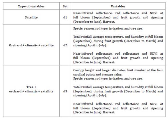
Noteworthy is that the variables in dataset d1 are the cheapest, while, conversely, certain features in d3 are quite expensive as they rely on human resources.
Methods to estimate orchard production
ANNs are machine learning algorithms inspired by brain neural networks. They are widely used for both classification and regression tasks across various domains, including agriculture 9. One type of ANN is the multilayer perceptron (MLP), which consists of multiple layers of neurons. Each neuron receives input solely from neurons in the previous layer and provides output exclusively to neurons in the next layer. The first layer represents dataset input features, while the last layer represents the output. The number of hidden layers in between is typically determined through experimentation. During the training process, weights between adjacent neurons are adjusted to minimize prediction error. MLP has been applied in agricultural studies 27.
SVMs transform input data into a high-dimensional feature space using a predefined kernel function, wherein a hyperplane is derived to capture nonlinear relationships. SVM discovers this hyperplane by utilizing support vectors (essential training tuples) and margins (defined by the support vectors). Even though SVMs interpretation can be complex, they have been applied in agriculture with high accuracy 15,35.
RT adopt a divide-and-conquer strategy to construct a tree. Each path from root to leaf determines a region representing a more homogeneous subset of the input data. Various existing regression tree-based models are characterized by different splitting criteria, prune rules, and methods for estimating leaf values. CART uses variance as the splitting criterion, M5 employs standard deviation reduction, and conditional trees utilize covariance. In CART and conditional trees, the estimated value for a leaf remains constant, while M5 approximates it using linear regression models 21. In general, M5 outperforms CART and conditional trees in terms of accuracy and simplicity. These models have been extensively used in agriculture 7,20.
Random Forest (RF) constructs decision trees by repeatedly sampling the original training data through bootstrapping. Each decision tree is trained on a different random sample, resulting in trees trained on slightly different data subsets. RF combines the individual decision trees by averaging their predictions, reducing variance in predictions and improving overall accuracy. By assembling a collection of decision trees, RF mitigates the risk of overfitting and enhances model generalization performance on unseen data 16.
Lazy methods (as KNN) are distance-based learning methods that predict output values based on the nearest neighbors in the training set, assuming all features used to describe the dataset are relevant, and that close examples are likely to have the same output value. It computes distances (Euclidean or other) between examples to classify each training example by selecting the k closest neighbors. Since based on distances, KNN is quite sensitive to sliding scale but can be useful when interpretability is not a requirement for modelling a prediction problem 12.
Training and testing
Each dataset was divided into training and test sets, with a split ratio of 75% for training and 25% for testing. This process was repeated 50 times, ensuring unbiased results. The training phase followed a cross-validation model with 10 folds. The tested methods included M5, conditional trees (ctree), CART (implemented as rpart and rpart2), SVM with polynomial kernel (svm1) or radial kernel (svm2), perceptron with one layer (mlp) or two layers (mlpMP), k-nearest neighbors (knn), and random forest (RF).
Model performance was assessed through various metrics, including the root mean square error (RMSE), commonly used for validating physical system models 6. It is defined as follows:

where:
n = the sample size
i = the output value and u is the prediction
The mean absolute error (MAE) quantifies the average difference between the measured data and the estimated data 17, quantifying error magnitude without considering direction. A lower MAE indicates a better model fit, and can be calculated using the following formula:

Results
Machine learning + datasets comparison
Different machine learning methods were assessed for prediction performance. Graph analysis indicated that random forest (rf) and SVM with polynomial kernel (svm1) had the lowest MAE and RMSE values. Across all datasets, svm1 consistently outperformed the other methods. Statistical significance was determined after conducting one-tailed t-tests to compare average MAE and RMSE differences for svm1 against all other methods. All comparisons showed significant values (p≤0.05), confirming that, for citrus production, svm1 had lower MAE and RMSE errors than other methods. The only exception was the RF comparison using dataset d1, showing no statistically significant difference in RMSE compared to svm1 (p=0.486). SVM with polynomial kernel (svm1) showed the best performance in terms of MAE and RMSE across all input datasets. Therefore, the analysis focused on evaluating svm1 performance.
Figure 2 shows the MAE vs. RMSE comparison obtained with svm1 using d1, d2 and d3 as inputs.

Figure 2: MAE (a) and RMSE (b) values obtained with svm1 for datasets d1, d2, d3. Figura 2: Valores de MAE (a) y RMSE (B) obtenidos con svm1 para los conjuntos de datos d1, d2 y d3.
Note that the worst performance was obtained with d1 dataset. A paired t-test compared d1 and d2 results and observed significant differences in MAE (p=1.757206-07) and RMSE (p=1.007665-06). Thus, d2 resulted the best dataset. On the other hand, d2 and d3 show small, non-significant differences (MAE (p=8.356207-01), RMSE (p=1.339823-01). Dataset selection was based on the variables used, considering measurement difficulties and costs. Given tree variables were the most difficult and expensive to collect, dataset d2 was chosen for not including these variables. This combination method-dataset threw a prediction average error of 3.99% with 3.7 % standard deviation for fruit number estimation. This error results much smaller than the 10% and 46% obtained in maize yield estimation 20.
Analysis of relevant features
As previously demonstrated, the optimal combination for harvest prediction involves using dataset d2 and the machine learning method svm1. However, one SVM drawback is the complicated assessment of feature relative importance in model construction, besides the fact that there is no standardized approach for evaluating variable importance in SVM-based classification models.
Despite this limitation, investigating the most relevant variables in this context remains important. To this end, this research assumed that if SVM performance weakened when all variables except one were used for training, then that excluded variable was significant for model construction. To check this assumption, the training used all variables except the one being considered, obtaining the associated error (ei). Afterwards, each variable was ranked according to this errors, obtaining a ranking, ri. This process was repeated 50 times, obtaining 50 different rankings, then aggregated using scoring ranking rules and assigning each candidate with a score, finally obtaining variable importance. Although many different ways may obtain a consensus ranking 28,29,30,31,32, the Borda count is a quite simple convex-ranking-rule 8, already successfully applied similarly by Rúa et al. (2023) .
The 10 more important variables were species, age, irrigation, red reflectance in February and December, near-infrared reflectance in February and December, NDVI in December, rain during ripening, and humidity during fruit growth.
To check this “variable importance estimation”, svm1 was trained with a new dataset called d2-filtered, using only the 10 most important variables selected above. Figure 3 compares svm1 trained with d2 and with d2-filtered. Note that training svm1 with d2-filtered seems to reduce MAE and RMSE, although not significantly (MAE, p=0.05455, RMSE, p=0.2808).
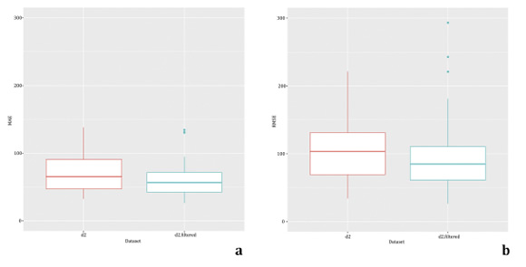
Figure 3: Comparison of MAE and RMSE using svm1 with d2 and d2 - filtered. Figura 3: Comparación de MAE y RMSE empleando svm1 con d2 y d2 - filtrado.
Thus, by using only these 10 most relevant variables, performance is not affected, and costs are reduced.
Discussion
This work evaluated several machine learning methods for low-cost orchard production estimation. These previously tested models determined volume, fruit number to harvest, or crop yield, using different remote sensors and yielding results in agreement with our research. RF and SVM resulted the best performance methods 14,15.
Leroux et al. (2019) compared a linear regression model with RF and found that RF outperformed the linear model and estimated maize yield two months before harvest using only data from the vegetative period. Han et al. (2019) explored four machine-learning regression methods (linear regression, SVM, ANN, and RF) modelling maize above-ground biomass using remote-sensing data.
ANN and SVM were considered difficult to interpret while the RF model gave the most balanced results, with low error and a high ratio of explained variance for the training and tested set. Feng et al. (2020) used machine learning-based integration with remotely sensed data to improve capabilities in monitoring agricultural drought.
Maya Gopal & Bharghavi (2019) evaluated features for accurate crop yield prediction and demonstrated that the RF model performed better. The variables used were planting area, number of tanks, number of tube wells and open wells, canal length for irrigation, amount of fertilizers consumed, seed quantity, cumulative rainfall, cumulative global solar radiation, and maximum, average and minimum temperatures.
Nyalala et al. (2019) developed a computer vision system for tomato volume and mass estimation based on depth images and several regression models. SVM showed significant advantages over other supervised learning algorithms. Kurtulmus et al. (2013) investigated various techniques for peach number estimation in a canopy, including SVM, ANN, and discriminant analysis. SVM demonstrated superior performance in certain scenarios, consistent with our findings. After evaluating multiple methods, RF and SVM with a polynomial kernel resulted the most effective, with the latter performing significantly better than other approaches across all datasets.
Figure 3 (page 71), shows harvest estimation using low-cost information related to species, season, tree age, soil type, irrigation, temperature, rain, and humidity, as well as satellite data at different moments. Begué et al. (2018) found similar results. Available literature on remote sensing for mapping cropping practices, concludes that testing at local scale is highly dependent on ground data. Robson et al. (2017) found a consistent positive correlation between vegetation index using near-infrared band 1 and red edge band with total fruit weight and average fruit size, concluding that orchard location and growing season influence this relationship. In the same line, Rahman & Zhang (2017) evaluated high-resolution satellite imagery for mango yield estimation by integrating tree crown area and spectral vegetation indices. They used ANN models, considering that the combination of these types of data allows estimating total fruit yield and fruit number with high accuracy. In addition, our estimation with almost 4% error for fruit number per tree, resulted in better fittings than those obtained by Leroux et al.(2019) . The method presented in this study represents an improvement over Bóbeda et al. (2018) , who relied on on-field information and the RT procedure to estimate fruit number in sweet orange and tangerine, with 29% error.
The 10 finally selected variables agree with previous research. Genotype and tree-age effects on citrus production are well-known and significant traits 25) for fruit number estimation in citrus. Concerning humidity, rainfall, and irrigation, plant optimal water intake is necessary for optimal plant growth and development. Kern et al. (2018) found an association between rain and yield in winter crops. NDVI and reflectance values for yield estimation resulted as previous yield predictors, based on the conclusions of Kern et al. (2018) and Lopresti et al. (2015) . In addition, noteworthy is that several of the most important features are measured during early crop stages.
Conclusions
This study presents a methodology using SVM for accurate estimations of fruit count per tree in Murcott tangor and Valencia late sweet oranges. The SVM model employs a polynomial kernel and considers several variables, such as species, tree age, irrigation conditions, rainfall during fruit maturation (April to July), humidity during fruit growth (December to March), red and near-infrared reflectance in February, and NDVI, near-infrared, and red reflectance in December. Easily obtainable ground variables, including species, tree age, and irrigation conditions, were recorded in each orchard. Meteorological stations provided rainfall and humidity data, while civilian satellites offered information. Estimations rely on low-cost variables obtained early in the determination process. The proposed estimation method enables safe and accurate anticipation of harvests at a reduced cost, demonstrating practicality and applicability.

