


 English (pdf)
 Article in xml format
 Article references
 Send this article by e-mail
 Cited by SciELO
  Similars in
SciELO
Similars in
SciELO 
 Permalink
INTRODUCTION
The CaCO3 determinations are standard analysis in Geology, Environmental Sciences and Soil Sciences, among other disciplines. Although many methodologies have been developed to quantify CaCO3 content, coulometric titration (e.g.,Engleman et al., 1985; Rowell, 1994; Kassim, 2013; Elfaki et al., 2016), oxidation by combustion (e.g.,Heiri et al., 2001; Wang et al., 2011, 2013), and CO2 pressure measurement after acid neutralization (e.g.,Sherrod et al., 2002; Stetson and Osborne, 2015) have been the most extended methods in Geosciences. These methods comprise low cost and time-consuming protocols, compared to more sophisticated techniques (e.g.,Zougagh et al., 2005; Tatzber et al., 2007; Gómez et al., 2008; Li et al., 2020). The CaCO3 type crystallinity (i.e., calcite, dolomite, aragonite), the expected content of CaCO3, the presence of organo-mineral components mixed in natural samples and the required data precision will determine the most suitable methodology in each case.
CaCO3 determination by Loss-on-Ignition (LOI) is a gravimetric method based on the CaCO3 decomposition by temperature which measures mass differences between combustion steps whose temperatures and durations vary significantly according to protocols (Dean, 1999; Heiri et al., 2001; Santisteban et al., 2004; Wang et al., 2011, 2013; Martínez et al., 2018). This method is indirect since combustion not only alters CaCO3, but also other components that also affect the final weight. For instance, important limitations arise when samples present abundant clays (e.g., illite, kaolinite, vermiculite, smectite), gypsum, oxyhydroxides (e.g., goethite), or any other H2O/OH-bearing mineral. The loss of structural water s.l. of such minerals, at 550 °C or even below, may generate an overestimation of mass differences (Moore and Reynolds, 1997; Heiri et al., 2001; Sun et al., 2009; Wang et al., 2011). On the other hand, the CaCO3 estimation by calcimetry is based on the CO2 pressure measurement after acid neutralization with HCl. Reaction occurs as follows:
CaCO3 + 2 HCl → CO2 + H2O + CaCl2
As observed with other methodologies, significant technical variations exist within calcimetry, including digital manometers with different types of glass chambers or the use of volumetric instruments such as the traditional Bernard or Scheibler calcimeters (Sherrod et al., 2002; Horváth et al., 2005). Independently of the instrument design, a well-known pitfall in calcimetry is the overestimation of CaCO3 content in samples with abundant organic matter (Hieri et al., 2001; Wang et al., 2011). Beyond this limitation, which can be controlled by addition of FeCl2 or FeSO4 (Loeppert and Suarez, 1996; Sherrod et al., 2002), it is noteworthy that the variety of chemical reactions taking place during acid neutralization inside the hermetic glass are better known than those produced under oxidizing conditions (LOI method) inside a furnace.
An important issue of any analytical determination derived from instrumental techniques is related to the limits of detection and quantification (Currie, 1995, 1999; ISO, 2000), information that is rarely provided by protocols. This is particularly important when analyzing low- CaCO3 content sediments (e.g., <4%), like the ones found in pedo-sedimentary and lake-core sequences (Dean, 1999; Zolitschka et al., 2000; Bockheim and Douglass, 2006; Doberschütz et al., 2014; Ozán et al., 2019; Li et al., 2020). In this context, the present work aims to present the critical value (LC), the detection limit (LD), and the quantification limit (LQ) of two pressure calcimeters that could be considered representative of instruments used worldwide, in order to propose a simple protocol to determine the CaCO3 content in natural samples with a low content of this compound, namely, below the LD and LQ of the instruments. In this regard, LD and LQ values were first calculated for both calcimeters and a series of essays were run with a pure salt pattern and natural samples. The CaCO3 content in the latter was also analyzed by LOI, so inter-method and intra-method results are discussed, as well as the applicability and pitfalls of calcimetry in low- CaCO3 content samples.
MATERIALS AND METHODS
Two pressure calcimeters were used to conduct the study: 1) the CALHH81, Netto S.E (series N°0921-8697, made in Argentina) (Fig. 1a), and 2) the Digital Gauge Calcimeter 2.3, Houston Mud Logging Supplies, LLC (series 4395, made in USA) (Fig. 1b). Instruments (hereafter referred as Netto and HMLS) were operated at room temperature (~20 °C) at the Chemical Laboratory of the Department of Geological Sciences at the University of Buenos Aires (Argentina). The Netto calcimeter measures the CO2 pressure generated from the dissolution of CaCO3 contained in a dry sample (1 g) when adding 20% HCl solution (20 ml) by using a piezoresistive sensor. The reaction takes place in a hermetic acrylic container of 500 ml, placed in a metal press. The glass is connected to the sensor equipment through a three-month valve, using a thin tube (143 cm length and 4 mm diameter) (Fig. 1a). Dissolution processes occur when the acid is manually decompartmentalized and mixed with the sample. After reaction, gases are released through the third valve orifice. An internal autocalibration converts pressure into percentage with a 0.1% precision. After ca. 45 seconds, measurements are stabilized, and gases can be released. The glass is then carefully washed and rinsed with milli-Q water. Once the instrument is turned on, an external calibration with 1 g of pure CaCO3 is needed to set 100% concentration, whereas the auto-zero is established before each measurement. In contrast to Netto, the HMLS design is alike others pressure calcimeters commercialized worldwide. Here, a digital manometer is attached to a hermetic acrylic container of 137 ml placed on a magnetic stir bar to favor the reaction. The HCl solution (10%, 20 ml) is injected with a luer lock syringe into the reaction chamber (Fig. 1a), where 1 g of dry sample is placed. After a 30-seconds measurement, gases are released. The glass is then carefully washed and rinsed with milli-Q water. A single external calibration is required to correlate the pressure value of the CO2 (PSI) with the concentration (%) of CaCO3 (precision 0.01 PSI). The auto-zero is stablished before each measurement.
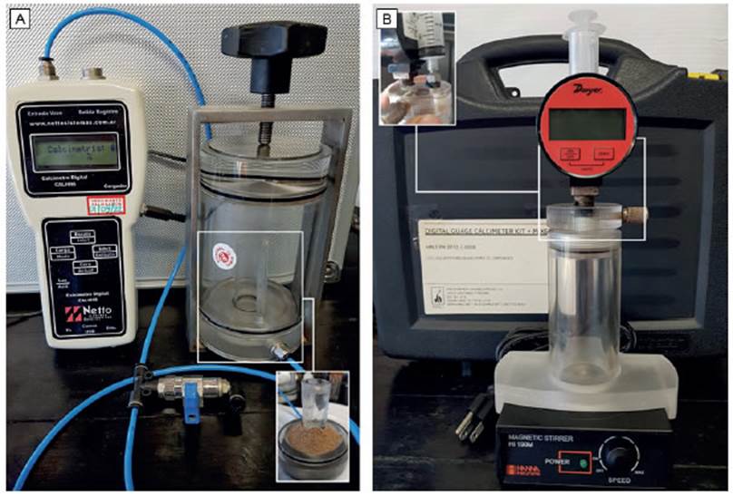
Figure 1 View of pressure calcimeters. a) CALHH81-Netto S.E (“Netto”), and b) Digital Gauge Calcimeter 2.3-Houston Mud Logging Supplies, LLC (“HMLS”).
External calibration curves
Instruments were calibrated using a CaCO3 standard of analytic quality (99.7%), dried during 12 hours at 105 °C and stored in a desiccator with silica gel (same protocol was followed for dry natural samples). Different proportions (in triplicate) of pure salt (0; 0.005; 0.001; 0.05; 0.1; 0.25; 0.5; 0.75; 1 g) were used to build the curve. A precision balance of 0.0001 g was used to weigh the pure salt and natural samples. The statistical analysis and linear regression fit were performed with Origin 9.0 Pro software.
Critical Value, Detection limit and Quantification limit
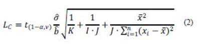
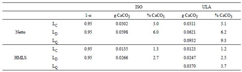
Three parameters were calculated for each calibration curve (i.e., LC, LD, LQ) following criteria of the International Organization for Standardization (ISO) and the Upper Limit Approach (ULA), recommended by the International Union of Pure and Applied Chemistry (IUPAC). The critical value (LC) is the minimum significant value of an estimated net signal (or concentration), applied as a discriminator against background noise. The comparison of an estimated quantity with the LC, such that the probability of exceeding LC is no greater than α if the analyte is absent, allows making the decision whether the net signal (or concentration) is detected or not (Currie, 1995, 1999; ISO, 2000). Assuming the results have a normal distribution with known variance, the LC can be described as:

where z1-α is related to the (1-α) percentage point of the standard normal variable and σ0 is the standard deviation of the blank. If the data have a normal distribution with a known variance and ν degrees of freedom, z1-α must be replaced by the t distribution parameter (t(1-α,ν)).
According to ISO (2000), this expression becomes:
where is the estimated residual standard deviation of the calibration curve, is the estimated value of the slope, K is the number of preparations for the actual state, I is the number of states (calibration standards) and J is the number of parallel measurements.
On the other hand, ULA (Mocák et al., 1997, 2009; Vogelgesang and Hädrich, 1998), describes the LC as:
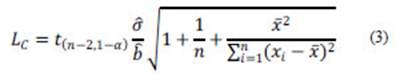
where n (equivalent to I·J, see eq. 2) is the total number of measurements.
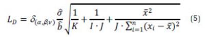
The minimum detectable value or detection limit (LD) of the net signal (or concentration) is the value for which the false negative error is β, given LC (or α) (Currie, 1995, 1999). It is the true net signal (or concentration) for which the probability that the estimated value does not exceed LC is β. Mathematically, when the distribution is normal and the variance is known, the LD is given as:
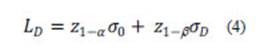
where σD is the standard deviation which characterizes the probability distribution of the signal when its true value is equal to LD. In case the variance is constant, σD is equal to σD and, based on ν degrees of freedom, z1-α + z1-β must be replaced by δ(α,β,ν), the non-centrality parameter of non-central-t distribution (Currie, 1995, 1999; ISO, 2000).
The expression for LD described by ISO (2000) is:
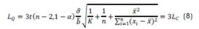
When α = β, δ(α,β,ν) is approximately equal to 2t(n-2,1-α).
The expression for LD suggested for the ULA is:

Finally, the limit of quantification (LQ) refers to the smallest net signal (or concentration), which can be quantitatively analyzed with a reasonable reliability by a given procedure (Currie, 1995, 1999). The ability to quantify is generally expressed in terms of the signal or analyte (true) value that will produce estimates having a specified relative standard deviation (RSD), commonly 10%. That is,
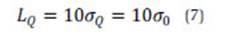
where σQ is the standard deviation at that point and 10 is the multiplier, whose reciprocal equals the selected quantifying RSD. If σQ is known and constant, then σQ in eq. (7) can be replaced by σ0. The various approaches to the LQ are somehow arbitrary. When using the ULA, the LQ is described by three times the LC:
It is noteworthy that detection and quantification limits refer to the capabilities of the measurement process itself and are not associated with any particular outcome or result (Bernal and Guo, 2014). On the other hand, the detection decision is result-specific, since it is made by comparing the experimental result with the critical value used to make a posteriori estimation of the detection capabilities of the measurement process, while the limit of detection is used to make an a priori estimate (Bernal and Guo, 2014).
Natural samples
Four natural samples from the Western Pampas Dunefield, province of San Luis, Argentina, (Zárate and Tripaldi, 2012; Tripaldi and Zárate, 2016) were considered for analytical essays (i.e., M3, M13, G1 and RC1). They correspond to Quaternary sediments recovered at different levels of aeolian sequences (i.e., vegetated dunes) with low-intensity pedogenesis/diagenesis (Tripaldi and Forman, 2007, 2016; Tripaldi et al., 2010, 2013; Forman et al., 2014). Well-sorted, fine-grained sands composed of volcanic lithics fragments, volcanic glass shards, and feldspars dominate the lithology of these sands (Forman et al., 2014; Tripaldi and Forman, 2016).
The clay fraction was measured by means of sedigraphy (Malvern Sedigraph). Structured thin sections for micromorphological descriptions and mineralogical optical quantification analyzed under a petrographic microscope (Zeiss, Axioplan 2) were also done at the same levels where the bulk samples used for calcimetry were taken (Stoops, 2003; Stoops et al., 2010; Ozán et al., 2019). Additional data concerning macroscopic characteristics of the sample (i.e., texture, structure, colour, context) were also reported (Folk et al., 1970; Munsell Color, 1994).
Pressure calcimetry in natural samples: After quartering, samples with concretions and/or aggregates were homogenised using a porcelain mortar. Since granulometry is <100 μm, the use of sieves was avoided. Samples were dried and weighted as mentioned above (see “External calibration curves”). The CaCO3 content of natural samples was estimated with the two different pressure calcimeters, following the corresponding protocols (see above, Materials and Methods). Since the evaluated signals for 1 g of each sample were often lower than the LD and/or LQ, masses were increased gradually (“additional mass procedure”) until reaching results (% CaCO3) above the LQ (the amount of sample in the Netto calcimeter was limited by the chamber design; Fig. 1a). At least four measurements were performed for each sample and an accurate CaCO3 per g was then calculated.
Loss-on-Ignition in natural samples: Duplicate samples were ground with a porcelain mortar and weighted with a 0.001 g precision balance. About 3 g of sample was placed in porcelain crucibles a) to dry in oven for 12 hours (105 °C) and burnt in furnace at b) 550 °C and then c) 950 °C, for 2 hours in each combustion step (Heiri et al., 2001). Mass differences (in percentages) between each step gave the content of a) Water loose, b) Organic Matter, and c) CaCO3 (after applying the 1.36 convert factor). Calculation of the Organic Matter (%) and the CaCO3 (%) followed these equations (Heiri et al., 2001):
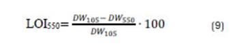
where DW represents the dried sample weight at different steps. Roughly, authors report an error of about 2% for LOI estimations.
The statistical analysis for the comparison of LOI950 and calcimetry results was conducted using a parametrical Two-way ANOVA test, followed by a Bonferroni posttest.
RESULTS
Calibration curves: LC, LD and LQ determinations
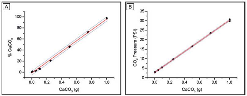
The linear regression for both calibration curves (Fig. 2) shows a determination coefficient (R2) above 0.997, which means that this model explains the 99.7% of the variance of these results (Table 1). In the case of HMLS, the linear fit is slightly better than the one for Netto, since the R2 value is not only higher but also residuals are normally distributed (Table 1, Fig. 3b).
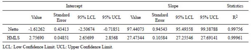
Table 1 Linear fit parameters of calibration curves for both calcimeters measured by LOI and pressure calcimetry with Netto and HMSL calcimeters.
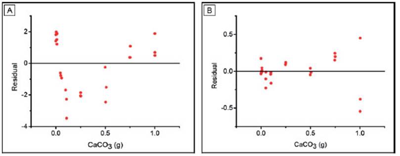
On the other hand, the residual plot for Netto shows a non-random pattern presenting a trend towards positive values for the low and high CaCO3 extremes, respectively (Fig. 3a). The comparison of LC and LD with both instruments shows no significant differences between ISO and ULA methods (Table 2). Limits calculated with Netto are nearly three times higher than those calculated with HMSL. In this sense, the Netto LC, LD and LQ are 3.1%, 6.2% and 9.3%, respectively, whereas in HMSL, those parameters are 1.2%, 2.5% and 3.7%, respectively (Table 2). Thus, the latter equipment shows better performance for low CaCO3 content determinations.
Natural samples: relevant characteristics and LOI determinations
The analyzed sandy sediments present a low organic matter content, between 1.5-2.7% and a variable proportion of clay fraction (0.5-4.3%). Concerning the CaCO3 content determined, results show values between 0.5-1.5%. Optical estimation of mineral composition (Table 3) shows that M3 and M13 samples mainly present plagioclase, followed by K-feldspar, lithic fragments (mainly volcanic), volcanic glass shards, and quartz, among other minor minerals. Sample G1 is mainly composed by lithics followed by volcanic glass, quartz, K-felspar, and opaques; whereas RC1 is dominated by K-felspar, opaques, volcanic glass, and plagioclase. Broadly, the well-sorted fine sands observed through the micromorphological examination of M3 supports the aeolian origin of the deposit (Forman et al., 2014; Tripaldi and Forman, 2016), with rare organic matter and the occurrence of diagenetic features represented by formation of authigenic clay minerals (e.g., illite) and the precipitation of amorphous Fe/Mn oxides (e.g., goethite) derived from the volcanic glass weathering (Fig. 4a). Sample M13 is similar to M3, but the thin section does not register the presence of organic matter remains, whereas it shows a crystallithic b-fabric, suggesting the presence of CaCO3 embedded in the matrix. Indeed, abundant nodules, stains, coatings, and hypocoatings of CaCO3, some of them with signals of dissolution and re-precipitation, are also observed (Fig. 4b).
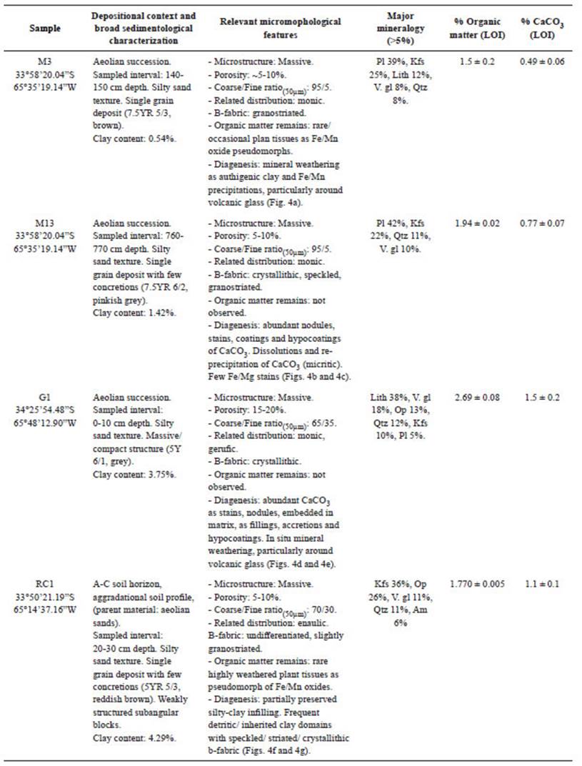
Table 3 Natural samples under study. Data expressed as mean ± standard deviation of duplicate samples. Lith = lithics; Pl = plagioclase; Kfs = K-felspar; V. gl = volcanic glass; Qzt = quartz; Op = opaques; Am = amphiboles.
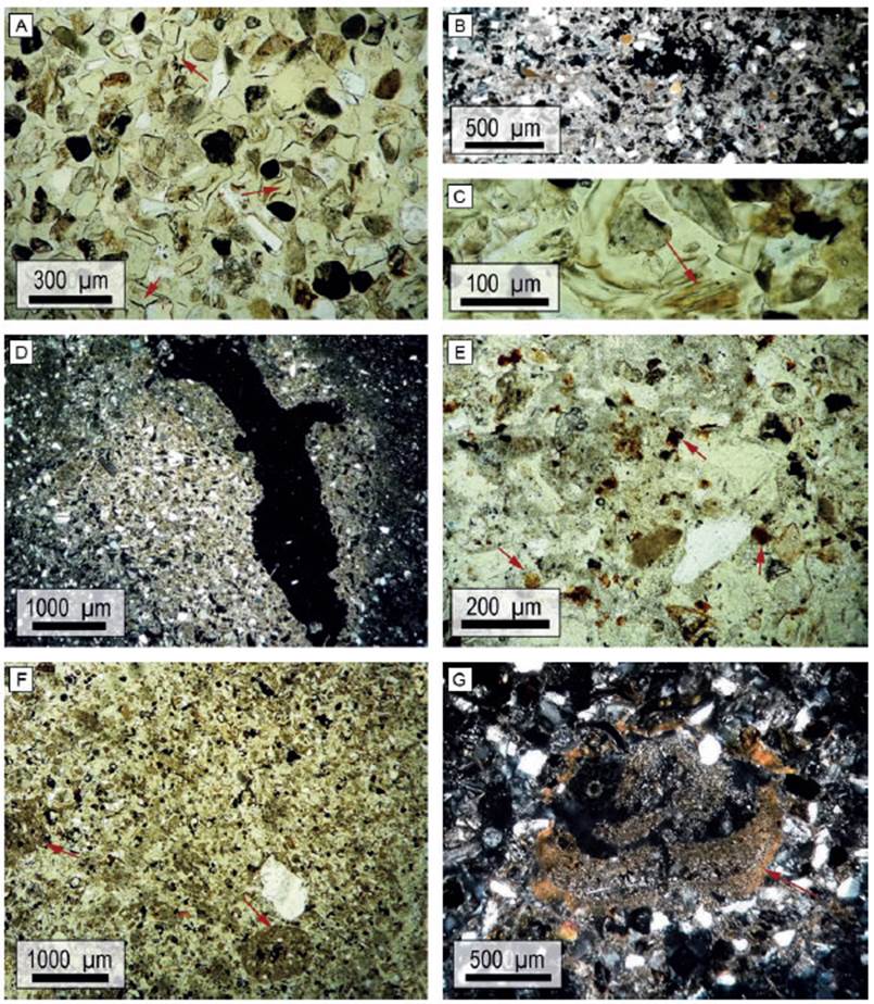
Figure 4 Microphotographs of structured thin sections corresponding to the four analyzed samples. a) Sample M3: massive, well sorted deposit of fine sands mainly represented by volcanic glass shards -indicated with red arrows- and highly altered lithics (Plane Polarized Light -PPL-). b) Sample M13: micritic CaCO3 embedded in the matrix (Crossed Polarized Light -XPL-). c) Close up of sample M13: Fe-oxide (e.g., goethite) because of in situ volcanic glass weathering (PPL). d) Sample G1: CaCO3 hypocoating with some Fe/Mn-oxide stains; crystallithic b-fabric (XPL). e) Close up of sample G1: Fe-Mn-oxide nodules (red arrows), stains and coatings around particles (in situ mineral weathering) (PPL). f) Sample RC1: well sorted silty sand deposit, undifferentiated b-fabric, and signals of soil fauna activity -pointed by red arrows- (PPL). g) Detail of sample RC1: void coating/ hypocoating of silty/clay, with crystallithic b-fabric (XPL).
In the case of G1, the micromorphology shows a relatively finer deposit with a lack of organic matter but abundant amorphous CaCO3 as stains, nodules, infillings, accretions, and hypocoatings (Fig. 4d). In situ mineral weathering, particularly around volcanic glass (e.g., goethite) is also registered (Fig. 4e). Alike G1, RC1 sample shows a loamy deposit (Fig. 4f), which includes silty-clay void infillings and frequent detritic clay domains with speckled/ crystallithic b-fabric (Fig. 4g). Rare plant tissue remains are observed as pseudomorph of Fe/Mn oxides and the undifferentiated b-fabric (Fig. 4f) may suggest the presence of highly degraded organic matter (i.e., humus).
CaCO3 by pressure calcimetry in natural samples by applying the “additional mass procedure”: The amount of % CaCO3 per g of sediment sample considered an “accurate” result is an average of % CaCO3 per g of measurements which yielded values above the LQ. Thus, reliable results are observed in three samples using both instruments, but not in M3. The high LC value calculated for Netto (3.1%), prevented this calcimeter to detect the very low content of CaCO3 in sample M3, not even with 12 g, the maximum volumetric limit of the glass (Fig. 1a). Similarly, the LD could not be reached with the HMSL for 12 g of sample M3 because a technical limitation of the instrument.
DISCUSSION
First, two main relevant issues arise from the calculation of the LC, LD and LQ values: 1) HMLS is a more sensitive calcimeter, thus showing lower values for these parameters, and 2) instruments do not accurately detect CaCO3 content below their LD, namely, 2.5% (HMLS) and 6% (Netto) (Table 2), so results challenge data robustness for low-CaCO3 content samples. The more accurate results obtained with HMLS calcimeter are probably related to its smaller reaction chamber and the manometer being directly attached to the glass, a fact that simplifies the equipment by avoiding internal calibrations that may add another source of error. It is important to outline here that both instruments display a result even when measurements fall below the LD, so users can obtain unreliable measurements if LC, LD and LQ are unknown.
Pressure calcimetry measurements with 1 g of natural sample were lower than LQ values, so a higher mass of sediment was gradually added until obtaining results above that limit (9.3% and 3.7% for Netto and HMLS calcimeters, respectively) (Table 2). Consequently, the amount of CaCO3 corresponding to 1 g of sample was inferred (Table 5). This simple procedure proved to be successful in obtaining reliable results. Thus, in the case of the Netto instrument, if the expectation of CaCO3 content is below 9.3% (LQ), it is recommended to add ~10 g of sample and then normalize the result to 1 g. In the same way, with instruments like HMLS, which are more representative of worldwide designs, when samples with CaCO3 content below 3.7% are expected, ~4 g samples should be used to obtain accurate values. Whereas this procedure increases the scope of the calcimetry methodology, the fact that it requires a high amount of sample implies a disadvantage for some studies, like limnological analyses, where coring gives low-mass samples.
Despite of differences concerning instrumental designs and their LC/ LD/ LQ thresholds (Fig. 1, Table 2), both calcimeters yielded similar results of CaCO3 in natural samples, though the very low CaCO3 content of M3 could not be measured by any instrument, not even by the “additional mass procedure”. Interestingly, micromorphological analysis did not show the presence of CaCO3 on M3, therefore, the lack of accurate measurements in calcimetry could be related to a “real” absence of CaCO3 in this sample. On the other hand, the abundance of CaCO3 (estimated qualitatively) in thin sections of M13, G1 and RC1 samples support the amount of CaCO3 content determined by calcimetry (Table 3). Comparations between calcimetry results and the LOI method indicate rather similar values between both techniques (Table 5), except for G1. For M3 sample (undetectable in calcimetry), a ~0.5% of CaCO3 was determined by LOI. However, as mentioned, the absence of CaCO3 in the thin section may suggest that the value is not reliable for the method and/ or it is a consequence of other processes that occurs with burning, such as mineral water loss and mineral dehydroxylation at temperatures above 550 °C (e.g.,Moore and Reynolds, 1997; Wang et al., 2011). Even though non-significant differences in CaCO3 content are observed in M13 and RC1 samples comparing the two methods (Table 5), slightly lower values in LOI (~23%) could be attributed to an overestimation of organic matter by LOI determinations, a fact that later impacts on CaCO3 estimations (eq. 10). Similar arguments may explain the significant difference between calcimetry and LOI CaCO3 estimations obtained for G1 sample, which yielded a below-50% value in LOI (Table 5) (c.f., Li et al., 2020). Here, while LOI analysis shows a relatively higher amount of organic matter compared to the other samples, micromorphology does not register the presence of any tissue remain not highly degraded organic matter such as humus. In addition, G1 sample presents the highest percentages of volcanic glass, whose weathering subproduct could be assigned to goethite, a mineral that suffer dehydroxylation above 300 °C (Sun et al., 2009; Gialanella et al., 2010). Indeed, geochemical analyses applied on the volcanic glass of the region supports the formation of such oxyhydroxide (Toms et al., 2004; Tripaldi et al., 2010).
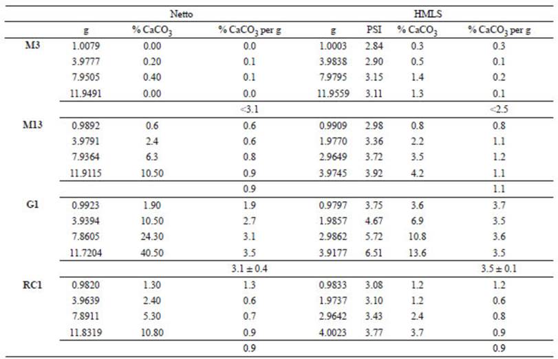
Table 4 Pressure calcimetry by Netto and HMSL calcimeters, applying the “additional mass procedure”.
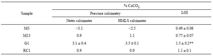
Table 5 Synthesis of CaCO3 content measured by LOI and pressure calcimetry with Netto and HMSL calcimeters. Significant differences between methods are given by two asterisks with a P value less than 0.01.
In sum, pressure calcimetry is a fast CaCO3 determination method (over 20 samples can be run in one hour work) with reliable results if the LC, LD and LQ are calculated, as they are highly significative values for users. Furthermore, this analysis shows that when low-CaCO3 content samples are under study, increasing the mass of sediments may help improve the sensibility of the instrument. Calcimetry results in the set of natural samples also show consistency with micromorphological analyses and, except for a few differences, LOI method.
CONCLUSIONS AND RECOMMENDATIONS
A simple protocol to obtain robust CaCO3 determinations through pressure calcimetry in low- CaCO3 samples (<4%), even though their CaCO3 content falls below the limit of detection of the instruments, was validated by mean of calculations of the critical values (LC), detection limit (LD), and quantification limit (LQ) for two different pressure calcimeter instruments. Then, a set of four natural samples with low-CaCO3 content were measured with both calcimeters to prove the utility of such calculations. The LC, LD and LQ (95% confidence) were 1.2%, 6.2% and 9.3%, respectively, for the Netto instrument (Argentina); and 1.2%, 2.5% and 3.7%, for the HMLS instrument (USA), respectively. Determinations of CaCO3 by LOI and micromorphological examinations were also conducted to expand the discussion of calcimetry results. Since CaCO3 content in natural samples was below the LQ calculated for pressure calcimeters, a simple “additional mass procedure” was conducted to obtain results above the LQ. Estimations of CaCO3 per g were afterwards recalculated. This analysis derived in the need of including 10 g and 4 g, for Netto-like and HMLS-like instruments, respectively, in order to ensure accurate results. Both calcimeters showed comparable results for natural samples and high consistency with micromorphological observations. In contrary, the latter analysis did not support the organic matter estimation by LOI (which could affect, in turn, CaCO3 estimations), nor the presence of CaCO3 in sample M3.

