Robust identification toolbox

M. C. Mazzaro^l, P. A. Parrillo^m, R. S. Sánchez Peña^H

^l Dept. of Electrical Engineering, PennState University, University Park, PA 16802, USA cmazzaro@gandalf.ee.psu.edu.

^m Automatic Control Laboratory, Swiss Federal Institute of Technology, CH-8092 Zürich - SWITZERLAND parrilo@aut.ee.ethz.ch.

^H University of Buenos Aires and CONAE, Av. Paseo Colón 751, (1063) Buenos Aires, ARGENTINA, ricardo@conae.gov.ar.

Abstract — In this paper we present a brief tutorial and a Toolbox for the area of Robust Identification, i.e. deterministic, worst-case identification of dynamic systems. The uncertain models obtained fit exactly the framework of Robust control, speciallyH1 procedures, if the control of the system is the objective. The use of several of the identification algorithms are illustrated by means of a simulated example of a flexible structure.

Keywords — Robust Identification, two stage algorithms, identification, identification, Mixed time/frequency identification, parametric/nonparametric identification.

I. INTRODUCTION

The area of Robust Identification has been originally proposed by Zames in the Plenary talk at ACC 1988, and the first papers appeared in Gu et al. (1989) for approximation and in Helmicki et al. (1991) for Identification. This methodology allows the computation of a family of models (the so called uncertain model) from experimental data and a priori information, which can be used as a first step in a Robust Control framework. It is therefore a deterministic, worst-case approach which describes families of models in terms of or errors. In particular, frequency domain Robust Identification methods produce a set of models with additive dynamic uncertainty (Sánchez Peña and Sznaier (1998); Zhou et al. (1996)) which can be used directly as the representation of a physical system which may be controlled by an controller. To produce structured dynamic uncertain models, these Robust identification procedures should be used over different input-output sets. In this case, control design methods as m –synthesis (Sánchez Peña and Sznaier (1998); Zhou et al. (1996)) may be used. If time domain Robust identification is applied to the physical system, controllers (Sánchez Peña and Sznaier (1998)) could be designed.

    In this context model uncertainty stems from two different sources: measurement noise and lack of knowledge ot the system itself due to the limited information supplied by the experimental data.

    Different types of identification algorithms have been developed in this framework. The case where the available experimental data are generated by frequency domain experiments leads to based identification procedures (see Gu and Khargonekar (1992), Chen et al. (1995) and references therein). Instead, if the available experimental data originate from time domain experiments identification procedures (see Jacobson et al. (1992) and references therein) are used. In Parrilo et al. (1996, 1998), a new Robust Identification framework that takes into account both time and frequency domain experiments has been proposed. Thus, the problem where "good" frequency response fitting (small error norm) leads to "poor" fitting in the time domain is prevented. Finally, in Parrilo et al. (1999) an extension of this mixed time/frequency identification procedure to the case of systems with a parametric component is presented.

   This paper presents a Robust Identification toolbox which implements many of the different techniques available in this framework. As an example there is an application to the problem of a flexible structure. The toolbox has been developed for MatLab, and is freely available from the Web Site of GICOR (Robust Identification and Control Group) at the University of Buenos Aires: //www.fi.uba.ar/laboratorios/gicor/. The uncertain models obtained from this methodology are compatible with the different synthesis methods available in the Robust Control, LMI and m –Analysis toolboxes.

    This toolbox implements almost all the state of the art methods in this area, although it inherits a few practical limitations from the theory and the algorithms used to implement it. In the first place, a common weakness of the Robust Identification framework is the conservativeness of the error bounds. Better bounds are possible by using optimization methods, at the expense of a heavier computational load. Also, the LMI based approach, which is related to interpolation methods, is limited by the number of experimental data points. A strong research effort is devoted to the area of optimization methods, in particular LMI's, therefore larger practical problems are expected to be solved in a reasonable time, in the future.

   An extense bibliography has been devoted to this subject during the last years. A complete survey of the area can be found in Mäkilä et al. (1995); Sánchez Peña and Sznaier (1998) and Chen and Gu (2000). Next section presents a brief tutorial on this subject, and sections III, IV and V provide a more detailed explanation of frequency and time domain identification algorithms as well as interpolatory procedures, respectively. Section VI details the Toolbox commands, and section VII illustrates the use of all previous algorithms by means of a flexible structure, from which (simulated) "experimental" data have been obtained. Finally some Conclusions are drawn in section VIII.

II. ROBUST IDENTIFICATION FRAMEWORK

Each Robust Identification procedure takes as input data both a priori and a posteriori information on the real system.

    The a priori information characterizes the set of candidate models S which should contain the system to be identified , and the class of noises N that affect the experimental data, through the parameters K, r and .

    We consider in this paper the class of discrete time, linear, stable and causal systems, whose frequency response H(z) is related to its impulse response h(k) through the standard Z-transform evaluated at :

(1)

Therefore, analytic functions inside the unit circle represent causal and stable systems.

    In the case of frequency domain identification, the a priori class of candidate systems S is defined as:

(2)

This set contains all exponentially stable systems, i.e., those that satisfy the following time domain restriction:

(3)

with a worst-case gain to complex exponential inputs of K and a stability margin of (r – 1).

    In the case of time domain identification, the a priori class of models F results:

(4)

which includes the subset of systems satisfying (3) when and .

    If it is assumed that the system to be identified has the following structure:

(5)

where H_p(z) and H_np(z) represent its parametric and nonparametric components respectively, the a priori class of models T is defined as:

(6)

with:

(7)

and where the N_p components of vector G(z) are known linearly independent functions that satisfy the separation condition:

(8)

which guarantees that the decompostion (5) is unique (Parrilo et al. (1999)).

   The a priori classes of noises that are present during the frequency and/or time domain experiments, N_f and N_t, are:

(9)

The a posteriori information is a finite set of data y = E(,h) Î C^N, obtained from frequency domain ⁽¹⁾ or time domain experiments and corrupted by noise.

    The frequency domain data y^f Î C^Nf consist of a set of N_f samples of the frequency response of the system H(z), with additive noise h Î N_f :

(10)

which satisfy the following relation of complex conjugate symmetry (for N_f even):

(11)

with and real samples, as they proceed from a real rational system.

    The time domain data consists of the first N_t samples of the time response of the system to a known but otherwise arbitrary input, y^t Î , affected by additive noise:

(12)

where is the Toeplitz matrix of the input sequence, and h is a column vector with coefficients of the impulse response of the system.

    As output, a Robust Identification procedure provides a nominal model based on the a posteriori experimental data, and a worst-case bound e_id on the identification error, defined in an appropriate norm over the a priori set of candidate models.

    Thus, the family of identified models "covers" the set S(y) of all plants in the a priori class, which could have produced the a posteriori information with the class of noises assumed a priori:

(13)

and it should contain the real plant. This fact justifies the need to define a priori classes of models and noises. Otherwise all possible combinations of plants and noises which could have produced the experimental data, would form an unbounded set S(y) and the Robust Identification problem would make no sense, since e_id ® ¥ and could be any model.

    Finally, due to the fact that the assumed a priori information –the parameters K, r and – is a quantification of the engineering common sense, there is no guarantee that it will be coherent with the experimental a posteriori information. Therefore, consistency between both types of information should be tested, i.e., if the set (13) contains at least one element, before the application of a Robust Identification procedure. Otherwise, the worst-case bound e_id obtained over the family of identified models would be no longer valid. A discussion about the selection of the a priori data can be found in Mazzaro et al. (2001).

III. FREQUENCY DOMAIN IDENTIFICATION

A. Experimental Data

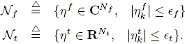
Given an experiment in the frequency domain, (9) and (10) provide at each sampling frequency q_k a ball in the complex plane of center and radius _f , which contains the true frequency response sample (Helmicki et al. (1991)):

(14)

if the assumed a priori bound on the measurement noise _f is "correct". Moreover, by performing M identical experiments a set of M balls centered at ( )i with radii (_f )_i for i = 1, 2, . . ., M will be obtained at each sampling frequency. Within the intersection of all these balls lies the real frequency response sample.

    By repeating and intersecting the experiments it is possible to obtain a smaller region which contains the real value, , i.e.,a smaller noise error bound h_k, reducing thus the worst case identification error eid(h_k, K, r).

    Figure 1 shows the result of the proposed procedure, for M = 3 experiments in the frequency domain at a generic sample frequency q_k. Due to the lack of an analytical expression for the intersection zone, this one is "covered" by the smallest ball of radius r_k and center c_k. Hence, c_k and r_k are taken as the resulting frequency response sample and the error bound respectively, at the frequency q_k. ⁽²⁾

Figure 1: Intersection of the experiments at a generic sampling frequency q_k.

B. Two stage Algorithm

This class of algorithms for identification in – developed in Helmicki et al. (1991); Gu and Khargonekar (1992)– are characterized by a two stage structure.

    The first stage involves taking the inverse discrete Fourier transform (DFT) of the frequency response samples:

(15)

considering only the first N_f coefficients of this real and periodic sequence, which gives a first finite approximation (FIR) to the impulse response of the real system:

(16)

and multiplying (16) by a suitable window function w(k) of length 2n + 1 with n = n(N_f ), in order to establish its convergence in , which yields the following preidentified model:

(17)

But due to the presence of measurement noise and to the fact that the real impulse response is in general of infinite length (IIR), the approximation obtained above (17) has a noncausal portion (negative Fourier coefficients), and therefore is non analytic inside the unit circle.

   The second stage involves solving the Nehari's problem, i.e., finding the optimal in analytic approximation for the pre-identified model obtained during the first stage (Glover (1984)).

   As the worst-case identification error after the Nehari's approximation is at most twice the error obtained in the first stage, the selected window function determines the type of convergence of the two stage nonlinear algorithm. Note that no a priori information is used to obtain a nominal model, thus this is an untuned identification procedure.

IV. TIME DOMAIN IDENTIFICATION

In this section, two time domain identification algorithms –developed in Jacobson et al. (1992)– are presented, which obtain a nominal model with impulse response h_id(k) = ()_k based on both a priori and a posteriori information, and which use the norm to quantify the worst-case identification error ⁽³⁾.

   1^st Algorithm: Given the a priori parameters K, r and , and the a posteriori experimental impulse response samples y_k, define the intervals:

(18)

where h_L(k) and h_U(k) represent the least and the greatest values of the impulse response h(k), which are consistent with the a priori information:

		(19)
		(20)

This algorithm (K, r, )selects for each k the center of these intervals, of length at most min():

(21)

2^nd Algorithm: Given the a priori information K and r, and the a posteriori information y_k, this algorithm (K, r) defines as the identified impulse response:

(21)

If the assumed parameters K and r are consistent with the experimental data y_k, h_id(k) is an interpolating model as it can generate the time domain data within the noise level assumed a priori.

V. INTERPOLATORY LMI BASED IDENTIFICATION

This identification framework –developed in Sánchez Peña and Sznaier (1995); Parrilo et al. (1996, 1998, 1999)– combines both frequency and time domain experimental data, and can be applied to the case of parametric/nonparametric model structures.

   Given the a priori class of systems T , the a priori classes of noises N_f and N_t, and the a posteriori frequency response and impulse response data y ^f and y ^t, determine:

• if the a priori information is consistent with the a posteriori information, i.e., if the consistency set T (y ^f , y ^t) (13) is non empty.
• a nominal model in the consistency set.

   The problem of checking consistency between a priori and a posteriori information reduces to finding a model H(z) = H_np(z) + H_p(z) in the a priori class of systems T , that interpolates the frequency and time domain a posteriori samples within the a priori noise levels. To solve this problem, a generalized interpolation framework presented in Ball et al. (1990) is used, which reduces to a Nevanlinna-Pick problem in the frequency domain case and to a Carathèodory-Fejèr problem in the time domain case. The main result of Parrilo et al. (1999) (see definitions and references therein) states that the a priori information is consistent with the a posteriori information, if it is possible to find three vectors w, h and p of appropriate dimensions, which satisfy the following restrictions:

		(22)
		(23)
		(24)

where (w,h) depends on both the a priori and a posteriori information, and the matrices _f and _t are functions of the experimental data from the assumed parametric component. These restrictions can be rewritten as a set of linear matrix inequalities (LMI's) in the variables w, h and p, and efficiently solved via convex programming algorithms (Boyd et al. (1994)).

Once consistency between a priori information and a posteriori time/frequency experimental data is established, this identification procedure provides a set of nominal models parametrized in terms of a free parameter Q(z) (see definitions in Parrilo et al. (1996, 1998)):

(21)

If the function Q(z) is chosen to be constant, the order of the identified nonparametric model is less than or equal to (N_f + N_t).

VI. ROBUST IDENTIFICATION TOOLBOX -ROBIT

A. Main Functions

In this section we present a brief description of the main functions of this toolbox. The background on these procedures can be found in the selected bibliography.

• freqsets: Finds the intersection of M sets of experiments of length N_f , performed in the frequency domain and corrupted by additive noise (Helmicki et al. (1991)).
  
  [yf,ef]=freqsets(Y,E)

Inputs:

- Y(N_f ,M): experimental data in the frequency domain.

– E(1,M): bounds on the measurement noise for each experiment.

Outputs:

– yf: final data set.

– ef: final error data.

• timesets: Finds the intersection of M sets of experiments of length N_t, performed in the time domain and corrupted by additive noise (Helmicki et al. (1991)).
  
  [yt,et]=timesets(Y,E)

Inputs:

– Y(N_t,M): experimental data in the time domain.

– E(1,M): bounds on the measurement noise for each experiment.

Outputs:

– yt: final data set.

– et: final error data.

• alg2stg: Performs the discrete time "two stage" identification (Helmicki et al. (1991); Gu and Khargonekar (1992)).
  
  [sysc,sysap,eid]=alg2stg(Hn,en,K,rho, window,windpar,apptype)

Inputs:

– Hn(N_f ,1): N_f noisy experimental frequency response data, at discrete frequencies q_k equally spaced over the unit disk between 0 and p.

– en(N_f ,1): frequency dependent a priori error bounds, at each frequency q_k (optional).

– K,rho: a priori information on gain and stability margins of the real plant (optional).

– window: type of window function (optional). Four types of windows are available,

* 'splinwin': sine window for the spline based identification,

* 'trianwin': triangular window for the Cesaro sum based identification,

* 'coswin': cosine window for the 'second Bernstein procedure' based identification,

* 'trapwin': trapezoidal window, mixture of rectangular and triangular windows.

– windpar: parameters of the selected window function [Nwc Mwc] (optional), with:

* Nwc: length of its causal portion,

* Mwc: length of its rectangular portion (only required if window='trapwin' else Mwc=[]).

– apptype: type of analytic approximation to nonanalytic portion of pre-identified model (optional).

* 'one_step': non-analytic portion is zero,

* 'nehari_ap': Nehari's approximation,

* 'fir_ap': FIR approximation.

Outputs:

– sysc: discrete transfer function corresponding to the analytic portion of the pre–identified model, obtained by the first stage of the algorithm.

- sysap: discrete transfer function of the analytic approximation to the non-analytic portion of the pre-identified model; only if apptype is provided. Both sysc and sysap are expressed in ascending powers of z.

- eid: worst-case identification error; only if a priori information and window type and parameters are provided.

• discneh: Finds the discrete-time Nehari approximation, analytic in the open unitary disk, to a nonanalytic (anticausal) system (Glover (1984)).
  
  [sysneh,eneh]=discneh(hac)

Inputs:

– hac: vector with the coefficients of the non-analytic (anticausal) impulse response: hac(1,N_ac)=[h(–N_ac) . . . h(–1)].

Outputs:

– sysneh: transfer function for the discrete-time Nehari approximation, [num;den]in ascending powers of z.

– eneh: upper bound on the approximation error.

• nehari: Finds the continuous time Nehari's approximation to an unstable system (Glover (1984)).
  
  [sysneh]=nehari(sysunst,tol)

Inputs:

– sysunst: system matrix of the continuous-time unstable system.

– tol: tolerance used at model balancing step (optional; default: tol=10^–16).

Outputs:

– sysneh: system matrix of the continuous-time Nehari approximation.

• nehshuff: Finds the q-order FIR approximation to a discrete-time system, analytic in the open unitary disk (Kootsookos et al. (1992)).
  
  [sysap,eap]=nehshuff(sys,q,tol,N)

Inputs:

– sys: original system matrix.

– q: order of the FIR approximation.

– tol,N: numerical tolerance and number of iterations (optional, both used to stop algorithm; default: tol=10^–16, N=30).

Outputs:

– sysap: vector with the coefficients of the FIR approximation.

– eap: upper bound on the approximation error.

• err2stg: Computes the worst-case error for the implemented "two-stage" identification algorithm (Helmicki et al. (1991); Gu and Khargonekar (1992)).
  
  [eid]=err2stg(K,rho,ef,Nf,window, windpar)

Inputs:

– K,rho: a priori information on gain and stability margins of the real plant.

– ef(N_f ,1): frequency dependent a priori error bounds.

– Nf: number of frequency data points considered in the identification.

– window,windpar: type of window function used by the first stage of the identification and its parameters. See function alg2stg.

Outputs:

– eid: worst-case bound on the identification error.

• l1ident: Performs a discrete time identification in (Jacobson et al. (1992)).
  
  [hid,eid]=l1ident(data,rho,K,e,type)

Inputs:

– data(N,1): finite and corrupted portion of the impulse response of the system to be identified, of lenght N.

– rho,K: a priori information on stability margin and gain of the real plant.

– e(N,1): time dependent a priori error bounds, for each experimental sample.

– type: type of identification algorithm,

* type=1: tuned to all a priori parameters K,rho,e,

* type=2: tuned only to K,rho.

Outputs:

– hid(N,1): impulse response of the identified system.

– eid: worst-case identification error.

• errell1: Computes the worst-case error for the implemented `1 identification algorithm (Jacobson et al. (1992)).
  
  [eid]=errell1(K,rho,et,Nt,type)

Inputs:

– rho,K: a priori information on stability margin and gain of the real plant.

– e(N,1): time dependent a priori error bounds.

– Nt: number of data points considered in the identification.

– type: type of identification algorithm selected; see function l1ident.

Outputs:

– eid: worst-case identification error.

• interpol: Checks consistency between the a priori information –K, r and (_f, _t)– and the a posteriori experimental data (Parrilo et al. (1996, 1999)).
  
  [W,Hn,P]=interpol(rho,K,data_f,data_t)

Inputs:

– rho,K: a priori information on stability margin and gain of the real plant.

– data_f: frequency domain data [Z Yf Ef Pf], with:

* Z(N_f ,1): discrete sampling frequencies,

* Yf(N_f ,1): frequency response measurements,

* Ef(N_f ,1): frequency dependent a priori error bounds,

* Pf(N_f ,N_p): parametric information matrix, Pf(i,j)=g_i(k) , i = 1, . . ., N_p (optional).

– data_t: time domain data [Ut Yt Et Pt], with:

* Ut(N_t,1): discrete time input,

* Yt(N_t,1): discrete time output,

* Et(N_t,1): time dependent a priori error bounds,

* Pt(N_t,N_p): parametric information matrix, Pf(i,j)=g_i(k) , i = 1, . . ., N_p (optional).

Outputs :

– W(N_f ,1): frequency response samples of the interpolating function H(z), i.e., H(z_i) = W_i.

– Hn(N_t,1): impulse response samples of the interpolating function

– P(N_p,1): coefficients of the parametric portion of the identified model.

• interp_e: Checks consistency between the a priori information –K and r – and the a posteriori experimental data, minimizing the a priori error bound = sup(_f, _t) (Parrilo et al. (1996, 1999)).
  
  [W,Hn,e,P]=interp_e(rho,K,data_f, data_t)

Inputs:

– See function interpol.

Outputs :

– e: optimal value of .

– See function interpol.

• interp_k: Checks consistency between the a priori information –r and (_f, _t)– and the a posteriori experimental data, minimizing the worst-case gain K (Parrilo et al. (1996, 1999)).
  
  [W,Hn,K,P]=interp_k(rho,data_f,data_t)

Inputs:

– See function interpol.

Outputs:

– K: optimal value of K.

– See function interpol.

• intmodel: Finds a nominal model which interpolates the frequency and/or time data, found by any of the functions interpol, interp_e or interp_k (Parrilo et al. (1996, 1999)).
  
  [Sint]=intmodel(K,rho,Z,W,Hn,Q)

Inputs:

– rho,K: a priori information on stability margin and gain of the real plant.

– Z(N_f ,1): discrete sampling frequencies (input to any of the functions interpol, interp_e or interp_k).

– W(N_f ,1): frequency response samples of the interpolating function (output from any of the functions interpol, interp_e or interp_k).

– Hn(N_t,1): impulse response samples of the interpolating function (output from any of the functionsinterp_e or interp_k).

– Q: system matrix of the free parameter function Q(z).

Outputs:

– Sint: system matrix of one possible interpolating model.

• errorint: Computes the worst-case identification error for the parametric/nonparametric mixed time/frequency identification algorithm presented in (Parrilo et al. (1999))
  
  [eid]=errorint(K,rho,Z,ef,Ut,et,Pf,Pt, Ginf)

Inputs :

– rho,K: a priori information on stability margin and gain of the real plant.

– Z(N_f ,1): discrete sampling frequencies.

– ef: a priori error bound in the frequency domain.

– Ut(N_t,1): discrete time input,

– et: a priori error bound in the time domain.

– Pf,Pt: a priori parametric information (optional; see function interpol).

– Ginf(Np,1): vector with the norms of functions that form the a priori parametric information (optional; only necessary if Pf,Pt are provided).

Outputs:

– eid: worst-case identification error.

B. Demostration Files

The demostration files show how to use the different functions of this toolbox. In all the examples, the "experimental data" –in the frequency and/or the time domain– proceed from the stable component of the Euler-Bernoulli model of a flexible beam with viscous damping, presented in Eqn. (26), section VII.

• demballs: Shows a procedure that can be applied to different sets of noisy data from the repetition of a single experiment, in order to obtain a smaller a priori error bound, reducing thus the worst-case identification error.
• dem2stg: Shows the discrete time "two stage" identification, with two options:

  1. Uses a trapezoidal window function at the first stage, and computes the Nehari's approximation at the second stage.
  
  2. User selection of the window function type, and the type of approximation to the nonanalytic identified system.

• demoell1: Shows the discrete time identification in , using two types of algorithms:

  1. Tuned to all a priori information K, r and _t.
  
  2. Tuned only to K and r.

• deminter: Shows the parametric/nonparametric mixed time/frequency identification, in the following cases:

  1. Identification in the frequency domain, considering only frequency response samples and no parametric component.
  
  2. Identification in the frequency domain, assuming that the real system has a parametric component with uncertain parameters.
  
  3. Mixed time/frequency identification, i.e., taking into account both frequency and time domain data (from the impulse response of the system), and considering a parametric component for the real model.

VII. APPLICATION EXAMPLE

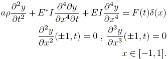
Next we illustrate the procedure explained above on a simulated example. The "real" system is an ideal Euler-Bernoulli beam with viscous damping, which can be described using the following physical model that relates the vertical displacement y to the time t and to the longitudinal coordinate x (see Fig. 2):

(26)

Here a is the cross sectional area, r the mass density of the beam, I the moment of inertia, E the Young modulus of elasticity and E* the normal strain rate. The dynamics are evaluated at x = 0 when a force F(t) is applied at this point. Due to the fact that the above PDE is linear, by using the Laplace transform an infinite dimensional transfer function can be derived (Klompstra (1987)). The discrete time model obtained by applying the bilinear transformation to the stable component (no rigid-body modes) has been used to simulate frequency and time domain experiments, with the following values for the constants of the model a · r = 46 kg·m, E*I = 0.46 kg ·m/sec and E · I = 55.2 N·kg (Mazzaro (1997)).

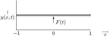
Figure 2: Application example: flexible structure.

A. Experimental data handling

Applying the function freqsets to a set of M = 3 identical experiments in the frequency domain, of length N_f = 50 and with noise bounded by _f = 8 · 10 ^–5 , the obtained frequency response samples and the new error bound–variable in frequency– can be seen in Fig. 3.

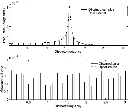
Figure 3: Results from the intersection of frequency domain experiments.

B. Two stage algorithm

Next, we apply this identification procedure to the physical system (26), using the programs of the Robust Identification toolbox. We consider 120 frequency response samples equally spaced in [0, p) (which gives N_f = 240 samples), proceeding from the intersection of M = 3 experiments corrupted by noise bounded by _f = 8 · 10^–5. During the first stage a trapezoidal window defined in Gu and Khargonekar (1992) as a function of the parameters m and n was used, with the values n + m = 120 (causal portion) and 2m = 60 (rectangular portion). This class of window function reflects through the ratio the trade-off between the approximation and noise errors, and allows to control its effects on the worst-case identification error.

    The function alg2stg performs the identification in one or two stages, as can be seen in Fig. 4. In the first case, the pre-identified model is taken as the identified one, which implies that the noncausal identified portion is approximated by the null function. Note that if N_f is large enough, the pre-identified model results a good approximation to the identified model, thus it is reasonable to neglect the noncausal identified portion. In the second case, the Nehari's approximation for the noncausal portion is obtained. It is also possible to compute a FIR approximation for the latter (Kootsookos et al. (1992)). In all cases, the function alg2stg allows to choose the type and parameters of the window function.

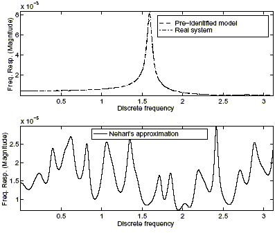
Figure 4: One or two stage identification.

C. Time domain algorithms

Next, we apply these identification techniques to the physical system (26), using the functions available in the Robust Identification toolbox. The experimental data proceed from the repetition and intersection of M = 3 experiments, which consist of the first N_t = 120 impulse response samples affected by noise bounded a priori by _f = 4 · 10^–6. The assumed a priori information on the class of systems are K = 4,5 · 10^–4 and r = 1.025. Function l1ident performs the identification in . The nominal model obtained with the first algorithm, tuned to all the a priori information, is shown in Fig. 5.

    The worst-case identification error (Jacobson et al. (1992)) for this algorithm is eid = 1.3787 · 10^–4, and can be computed using the function errell1.

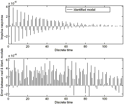
Figure 5: Identification in using the first algorithm.

D. LMI based algorithm

Next, we apply this identification framework to the physical system (26), using the different functions of the Robust Identification toolbox. We take into account N _f = 9 frequency response samples between [0, p], and the first N_t = 10 impulse response samples, corrupted by noise bounded a priori by _f = 8 · 10^–5 and _t = 4 · 10^–6, respectively. We also assume that the system to be identified has a parametric component with the following structure:

(27)

where p₁ and p₂ are uncertain parameters.

Figures 6 and 7 show the results of the identification in the frequency case without assuming a parametric component, and in the mixed time/frequency case with parametric component respectively, using the functions interp_k and intmodel. The first one finds the least value of the worst-case gain K, so that the a priori and the a posteriori information are consistent, and provides a set of frequency and/or time domain values to be interpolated by the set of nominal models. It is also possible to check consistency minimizing the a priori error bounds, using the function interp_e. The second one obtains an identified system for a given choice of Q(z). In both cases a value of r = 1.25 is assumed as a priori information, and the free parameter is chosen as Q(z) = 0. In the frequency case a value of K = 3.1465 · 10^–2 for the worst-case gain is obtained; in the mixed case, K = 3.8573 · 10^–4, p₁ = 4.1419 · 10^–4 and p₂ = –8.0218 · 10^–7.

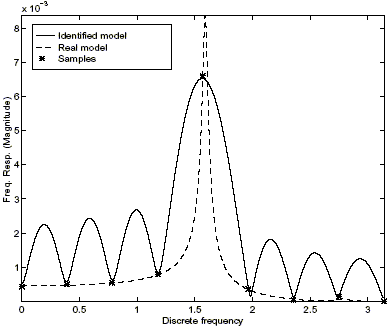
Figure 6: Frequency domain identification without parametric component.

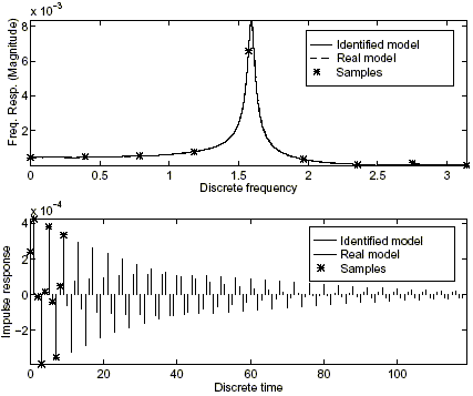
Figure 7: Mixed time/frequency domain identification with parametric component.

   This example illustrates the fact that, by adding a priori information –a parametric component– and a posteriori information –frequency and time domain data– smaller values of the gain K can be obtained, and thus, a "smaller" set of identified models (Parrilo et al. (1999)).

VIII. CONCLUSION

This work presents a Robust Identification toolbox, which implements the different identification techniques developed in the deterministic worst case framework, and which is not available as a commercial version.

    As an illustration, different procedures are applied to the problem of identifying a flexible structure of a known mathematical model, in order to evaluate the results obtained from the identification.

IX. Acknowledgments

The work of the first and last authors was supported by the UBACyT Project IN049, University of Buenos Aires and PICT Nº 1751 from ANPCyT. All authors would like to thank the useful comments of the reviewers.

¹ All the experiments are in fact performed in the time domain. Therefore the so called "frequency domain" experiments are carried out using sinusoidal inputs at different frequencies. A procedure to obtain frequency measurementsand its error bounds from time domain data is explained in Helmicki et al. (1991) in a Robust Identification framework.

² The application of this procedure to time domain experiments follows in the same manner as in the frequency case. At each discrete time one has a set of M real intervals, whose intersection zone can be computed exactly.

³ As the norm of a system with impulse response h(k) bounds the norm of its transfer function H(z) (Jacobson et al. (1992)): , identification in leads to identification in .

REFERENCES

1. Ball J., Gohberg I. and Rodman L., Interpolation of Rational Matrix Functions,Operator Theory: Advances and Applications, vol. 45, Birkhäuser (1990).         [ Links ]

2. Boyd S., Ghaoui L., Feron E. and Balakrishnan V., Linear Matrix Inequalities in System and Control Theory, vol. 15, SIAM Studies in Applied Mathematics, Philadelphia (1994).         [ Links ]

3. Chen J. and Gu G., ControlOriented System Identification An Approach, Wiley InterScience (2000).         [ Links ]

4. Chen J., Nett C.N. and Fan M., "Worstcase system identification in : Validation of a priori information, essentially optimal algorithms, and error bounds," IEEE Transactions on Automatic Control 40 1260–5 (1995).         [ Links ]

5. Glover K., "All optimal Hankel norm approximations of linear multivariable systems and their L^¥error bounds," International Journal of Control 39 1115–1193 (1984).         [ Links ]

6. Gu G. and Khargonekar P., "A class of algorithms for identificationin ," Automatica 28 299–312 (1992).         [ Links ]

7. Gu G., Khargonekar P. and Lee E.B., "Approximation of infinitedimensional systems," IEEE Transactions on Automatic Control 34 610–618 (1989).         [ Links ]

8. Helmicki A.J., Jacobson C.A. and Nett C.N., "Control oriented system identification: A worstcase/deterministic approach in," IEEE Transactions on Automatic Control 36 1163–1176 (1991).         [ Links ]

9. Jacobson C.A., Nett C.N. and Partington J.R., "Worst case systemidentification in : Optimal algorithms and error bounds," Systems and Control Letters 419–424 (1992).         [ Links ]

10. Klompstra M., "Simsat simulation package for flexible systems," Tech. Rep. 278, Dept. of Mathematics, University of Groningen (1987).         [ Links ]

11. Kootsookos P.J., Bitmead R.R. and Green M., "The Nehari shuffle: Fir(q) filter design with guaranteed error bounds," IEEE Transactions on Signal Processing 40 1876–1883 (1992).         [ Links ]

12. Mäkilä P.M., Partington J.R. and Gustafsson T.K., "Worstcase controlrelevant identification," Automatica 31 1799–1819 (1995).         [ Links ]

13. Mazzaro M.C., Algoritmos Numéricos Aplicados a la Identificación Robusta, Facultad de Ingeniería, Universidad de BuenosAires (1997).         [ Links ]

14. Mazzaro M.C., Parrilo P.A. and Sánchez Peña R.S., "Robust identification: A practical approach to select the a priori information," International Journal of Control 74 1210–1218 (2001).           [ Links ]

15. Parrilo P.A., Sánchez Peña R.S. and Sznaier M., "A parametric extension of mixed time/frequency robust iden  tification," IEEE Transactions on Automatic Control 44 364–369 (1999).         [ Links ]

16. Parrilo P.A., Sznaier M. and Sánchez Peña R.S., "Mixed time/frequency robust identification," Proceedings of the Conference on Decision and Control, 4196–4201 (1996).         [ Links ]

17. Parrilo P.A., Sznaier M., Sánchez Peña R.S. and Inanc T., "Mixed time/frequencydomain based robust identification," Automatica 34 1375–1389 (1998).         [ Links ]

18. Sánchez Peña R.S. and Sznaier M., "Robust identification with mixed time/frequency experiments: Consistency and interpolation algorithms," Proceedings of the Conference on Decision and Control, 234–236 (1995).         [ Links ]

19. Sánchez Peña R.S. and Sznaier M., Robust Systems Theory and Applications, John Wiley & Sons, Inc. (1998).         [ Links ]

20. Zhou K., Doyle J.C. and Glover K., Robust and Optimal Control, Prentice–Hall (1996)         [ Links ]

Received: August 29, 2002.

Accepted for publication: June 19, 2003.

Recommended by Subject Editor Oscar Crisalle.