Generation of orthorectified range images for robots using monocular vision and laser stripes

J. G. N. Orlandi and P. F. S. Amaral

Laboratório de Controle e Instrumentação (LCI), Departamento de Engenharia Elétrica (DEL),
Universidade Federal do Espírito Santo (UFES).
Av. Fernando Ferrari, s/n, CEP 29060-900, Vitória - ES, Brasil.
Emails: {orlandi,paulo}@ele.ufes.br

Abstract — Range images have a key role for surface mapping in robot navigation and control. The robot control system can easily identify objects and obstacles by manipulating range images, however most of these range images are acquired in perspective projection, thus object position may be incorrect due to distortion caused by the perspective effect. This paper proposes an easy and efficient way to acquire range images, with a single CCD camera in conjunction with laser stripes and afterwards these range images are orthorectified to turn out to surface maps. These orthorectified range images are very useful for biped and quadruped robots, orientating them when navigating among obstacles while robot manipulators can use them to find objects by setting up their joints and picking tools.

Keywords — Rangefinder; Robot Control; Vision System; Laser Stripes; Orthorectification.

I. INTRODUCTION

Range images are generally gray scale images whose pixel intensity represents elevation information of objects on a surface. A 3D surface reconstruction can be achieved if this surface has a range image.

This work proposes a computational, cost effective way to generate orthorectified range images compensating image perspective projection and radial lens distortion. Orthorectification aims to increase the precision especially for short distance images, where lens distortion and perspective effect are more visible.

In this paper, an active triangulation rangefinder has been developed using a monocular vision system composed by a CCD camera, calibrated for its intrinsic and extrinsic parameters and a laser, generating structured stripes on the surface for obtaining elevation information.

Bertozzi et al. (2000) described the pros and cons used for the detection of obstacles. He pointed out that stereo vision system is computationally complex, sensitive to vehicle movements and drifts and allows 3D reconstruction while optical flow, which is also computationally complex and sensitive to robot movements, demands a relative speed between robot and obstacles.

In this system, the computational time spent on generating the range images is lower if compared with stereo vision and optical flow techniques, thanks to the simplicity of the system modeling. This feature is fundamental for fast image processing serving the robot control system in a very satisfactory way.

There are several references for active triangulation laser rangefinders, some of them are mentioned here: Hattori and Sato (1995) proposed a high speed rangefinder system using spatial coded patters, Hiura et al. (1996) proposed a new method to track 3D motion of an object using range images, García and Lamela (1998) presented experimental results of a 3D vision system designed with a laser rangefinder, Haverinen and Röning (1999) presented a simple and low-cost 3D color-range scanner and Zheng and Kong (2004) introduced a method for calibration of linear structured light. For all these cited papers, there was no concern about the influence of image perspective effect on range images. This paper proposes an orthorectification process for correction of the perspective effect.

An application to the system is for a quadruped robot. The rangefinder has been assembled on Guará Robot (Bento Filho et al., 2004), which has 4 legs and each leg with 4 degrees of freedom. Figure 1 shows the system installed in front of the robot so that while the robot walks, scanned images from the surface are acquired and processed to generate the orthorectified range images.

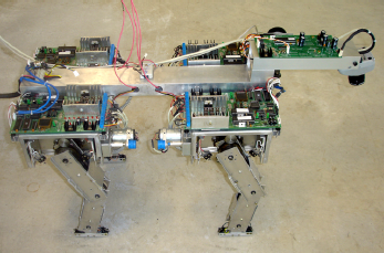
Figure 1: System assembled in front of Guará Robot.

The full system description and modeling, camera calibration, radial distortion correction, projective transformation, orthorectification process and laser stripes calibration are described.

Experimental results have shown that the system has a very good performance becoming a powerful tool for robot navigation.

II. SYSTEM DESCRIPTION

The system is formed by a color Pixelink^® CCD camera, set up for 1280x1024 image resolution in full field of vision, a 3.5 mW Class IIa laser stripe, a microprocessor board, a rotating mirror driven by a stepper motor. Figure 2 shows the acquisition system.

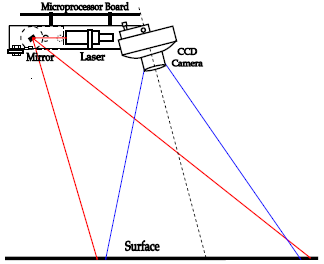
Figure 2: The Acquisition System.

The CCD camera is a Firewire (IEEE 1394) model, the frames are acquired and processed by a Microsoft^® Visual Studio .Net Windows-based application, using DirectX^® driver for fast acquisition. Besides, the microprocessor board based on Microchip^® PIC processor communicates with the application through USB, for laser control and other facilities. The Windows .Net application uses Visual C# as the programming language and runs on a 32-bit PC-based operating system.

The system basically controls the laser stripes and while they are projected on the surface, synchronized images are acquired to get the profile of the surface. These images are converted from RGB to grayscale, enhancing the red channel to increase the laser contrast.

The background image is removed, preserving only the laser stripe. The image is then binarized and skeletonized to have a thin and average laser stripe. This process is repeated for the amount of laser stripes and the more stripes the system processes the more precise range images are generated.

Figure 3 shows a specific region of interest of an image where all laser stripes are together. The number of laser stripes defines the resolution of the range image. Few laser stripes generate coarse range images while many laser stripes generate fine range images but it demands more processing.

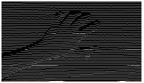
Figure 3: Laser Stripes on a surface region, scanning a hand and wrist.

III. SYSTEM MODELING

The system modeling is divided into two main parts: Camera Calibration: intrinsic and extrinsic parameters, mapping from surface to camera coordinates and Laser stripes Calibration: parameters to obtain elevation information from image pixels, therefore allowing generation of range images.

A. Camera Calibration

This section provides details of how to solve the camera calibration to recover the camera parameters which contain intrinsic and extrinsic parameters. Besides, camera lens radial distortion is modeled to suppress it and projective transformation is used to map surface plane into the image plane.

Intrinsic and Extrinsic Camera Parameters

Figure 4 shows the notation used to model a 3D point into a 2D point. P = (x_c,y_c,z_c) is a 3D point on the surface plane in the camera coordinates system, which is projected into p = (u,v) that is a 2D point of the image plane, S is the surface plane and I is the image plane. C is the optical center. Note that the image plane is virtually between C and S for making modeling easier, with f the focal length. The camera is modeled following the pinhole model.

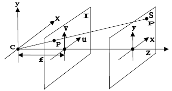
Figure 4: Pinhole Camera Model.

Let ^CP = [x_c y_{c c}]^T a 3D point on the surface in camera coordinates system and ^Cp = [u v 1]^T its 2D image projection, both in matrix notation. The relationship between ^CP and ^Cp is given by:

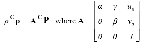(1)

Where ρ is an arbitrary scale factor, A is the camera calibration matrix representing the intrinsic parameters, (u₀,v₀) the coordinates of the principal point, α and β the scale factors in image for U and V axes respectively and γ the parameter which describes the skew of the two image axes, generally is zero.

The camera coordinates system is referenced to Guará Robot coordinates system, because the system is installed on it. Figure 5 depicts both coordinate systems, for simplicity only the camera is drawn.

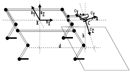
Figure 5: Guará Robot Coordinates System and Camera Coordinates System.

Let ^RP = [x_r y_{r r}]^T a 3D point in robot coordinates system, then:

^RP = ^RR_C ^CP + ^RT_C (2)

Where ^RR_C is the rotation matrix that encodes the camera orientation with respect to robot coordinates system and ^RT_C is the translation vector of the optical center to the robot coordinates system. Combining Eq. 1 and Eq. 2, then:

^RP = ρ ^RR_CA^{-1 C}p + ^RT_C (3)

^RR_C and ^RT_C can be also represented in a 4x4 matrix as follows (Zheng and Kong, 2004):

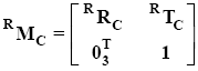(4)

Where ^RM_C is the matrix of the extrinsic camera parameters. For Fig. 5, ^RR_C and ^RT_C are respectively:

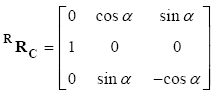	(5)
	(6)

Concerning the world coordinates system, it has to do with the Guará Robot control system.

Radial Distortion

Short distance images by wide angle lens exhibit significant distortion, especially radial distortion (Shu et al., 2005). This distortion is modeled to establish a relationship between pixels with distortion and pixels without distortion, expressed by:

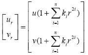(7)

Where (u_r, v_r) is the radial distorted pixel and (u, v) is the distortion-free pixel, and k₁, k₂,...k_n are coefficients for radial distortion. Dropping the higher order terms because they have small influence, considering k = k₁ the equation can be simplified and rewritten as follows:

(8)

Projective Transformation

Projective transformation, which is used in projective geometry, is the composition of a pair of perspective projections. It describes what happens to the perceived positions of observed objects when the point of view of the observer changes. Projective transformations do not preserve sizes or angles but do preserve incidence and cross-ratio.

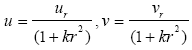
Projective transformation is the projection of one plane from a point onto another plane, being used in homogenous transformation where one coordinate in the surface plane is mapped onto one coordinate in the image plane. Figure 6 shows this transformation.

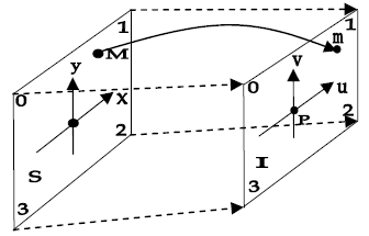
Figure 6: Projective Transformation.

Let M = [x y]^T a point on the surface plane S and m = [u v]^T its projective point on image plane I. Four known point on surface plane are referred to four known points in image plane. For this, the four corners of the image are chosen. The projective transformation has the aim to change the view point of the optical center, so that after the transformation, both image and surface planes become parallel and aligned, allowing to define the scale factors between both planes, as can be seen in Fig. 7.

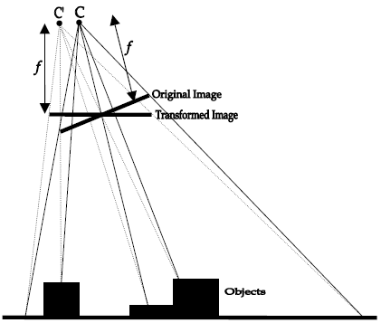
Figure 7: Changed optical center C' after projective transformation.

The projective transformation is a rational linear mapping given by (Heckbert, 1999):

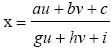	(9)
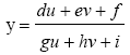	(10)

Where a - i are 9 coefficients for this transformation. Nevertheless, these equations can be manipulated to use homogeneous matrix notation becoming a linear transformation. For inferring this transformation, 4 fiducial marks (u_k, v_k) are chosen in the image and they are assigned to 4 known pairs (x_k, y_k) of the surface where k = 0, 1, 2, 3 and considering all coordinates are finite, thus i = 1.

In order to determine the 8 coefficients a - h it demands 8 equations as follows:

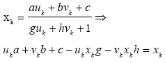	(11)
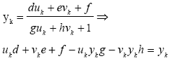	(12)

For k = 0, 1, 2, 3 in homogeneous matrix notation:

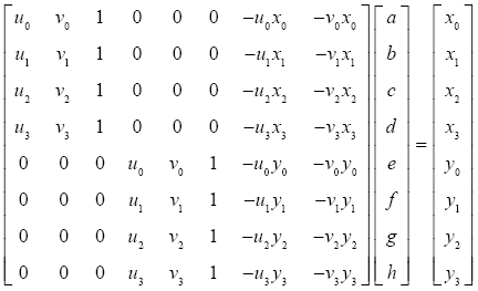(13)

This is a 8x8 linear system and the 8 coefficients a - h have been calculated by Gaussian elimination.

Figure 8 shows the calibration checker board plane, placed on the surface. In this case, Fig. 8 depicts the original image with radial distortion and perspective effect. This is the image before calibration.

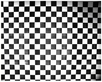
Figure 8: Checker Board before calibration.

Figure 9 depicts the same checker board plane after the calibration where both radial distortion and perspective effect have been suppressed.

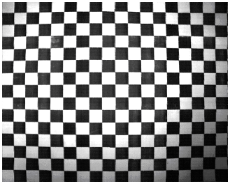
Figure 9: Checker Board after calibration using projective transformation.

After this transformation, the camera has been calibrated, hence each pixel image pair (u, v) have corresponding millimeter surface pair (x, y). In Fig. 9, each black or white mark has a 30x30 mm² area size.

B. Laser Stripes Calibration

Laser stripes are positioned on the surface, creating a structured light pattern. Figure 10 shows that any coordinate pair (x, y) from the surface is mapped into an associated coordinate pair (u, v) in the image plane. With incident laser stripes on the objects, it is possible to determine the elevation information z through triangle similarity between camera optical axis and the laser stripe. For object 1 whose height is h₁ and laser point is P₁ = (x₁, y₁, z₁) there is the image coordinate (u₁, v₁) and for object 2 whose height is h₂ and laser point is P₂ = (x₂, y₂, z₂) there is the image coordinate (u₂, v₂).

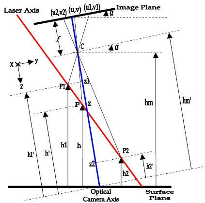
Figure 10: Laser-Camera Triangulation Modeling.

From Fig. 10, , and . The heights h₁ e h₂ are known and the height h can be found following the steps:

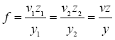(14)

Where f is the focal length. Any point in laser axis will satisfy the equation of a straight line which can be determine by the two points P₁ = (x₁, y₁, z₁) and P₂ = (x₂, y₂, z₂), then relating y and z:

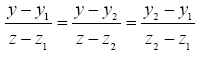(15)

Replacing y, y₁, y₂ from Eq. 14 in Eq. 15:

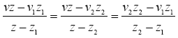(16)

Separating from Eq. 16 two constants: k = v₂z₂ - v₁z₁ and d = z₂ - z₁ obtaining z:

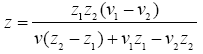(17)

Where n = z₁z₂ (v₁ - v₂) is also a constant, replacing the 3 constants in Eq. 17, this equation is simplified as follows:

(18)

However, since there is a pitch angle α between camera and surface planes, and the heights are measured perpendicular to surface, thus 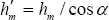, , e , the height h of a unknown object is given by:

h = h_m - zcosα (19)

C. Orthorectification

Cameras generate perspective images, it means that the light rays come from different image points and they all pass through a point called perspective center, which is the optical center of the camera.

As a consequence of this conic perspective, higher objects are seen bigger than they really are because they are closer to the camera.

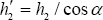
In orthogonal projection, the rays are projected from image in parallel, eliminating the distortion caused by the conic perspective. Figure 11 shows a drawing of 3 objects of different heights in perspective and the same 3 objects in orthogonal projection. In this drawing, the highest object is B and its gray level is closer to white. Note that after this process objects A, B and C get small, with their real dimensions.

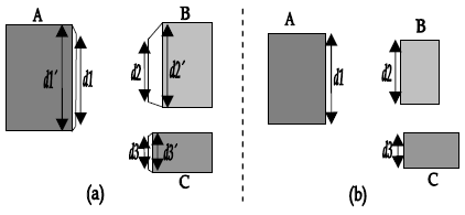
Figure 11: (a) Objects in Perspective (b) Objects in Orthogonal Projection.

The elevation information of the surface is prerequisite for orthorectification and it could be acquired from a DTM (digital terrain model) which represents not only coordinates of image area but also the altitude of the regions (Qin et al., 2003). In this system, elevation information is obtained from the lasers stripes on the surface. The process becomes simple once perspective range images are generated by CCD camera and laser stripes. Figure 12 depicts the suggested orthorectification process, applied to the perspective range images:

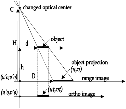
Figure 12: Orthorectification process.

Note that the changed optical center C' and principal point are due to the fact that the image has been corrected by the projective transformation, becoming its plane perpendicular to the surface plane.

By triangle similarity and considering that both range image and ortho image have the same dimension, the following equations are obtained:

	(20)
	(21)

Where (u, v) represents a point in perspective range image, while (u_t, v_t) represents its corresponding point in ortho image, H is the height from changed optical center C' up to surface plane, h is the height of any object, is the changed principal point for both images.

IV. EXPERIMENTAL RESULTS

In order to generate orthorectified range image, the surface area has been defined with 540 mm width by 450 mm height and it is mapped in a frame whose dimension is 640 pixels width by 512 pixels height during camera calibration. Several objects have been used to test the system, especially objects with the same area by different heights.

An average error has been estimated. The error is referred to surface dimensions. If the laser stripes, on an object, are closer to the camera, the image laser profiles will have higher values if compared with the laser stripes far from the camera, on the same object. So, the average measured error varies from ±0.5%, for closer objects to ±2.5%, for far objects. Far objects have more influence of the radial distortion and the image geometric transformations.

The camera optical center was installed 500 mm above the surface plane. Figure 13 depicts a original grayscale image of 5 objects and the laser stripe, Fig. 14 shows the same image with radial distortion and perspective corrections, Fig. 15 depicts the laser stripes on the surface, Fig. 16 shows the perspective range image and finally Fig. 17 and 18 show the orthorectified range image in top view and 3D view.

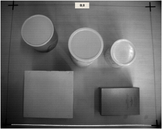
Figure 13: Original image of the surface with 5 objects and the laser stripe below.

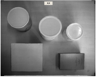
Figure 14: Image after radial distortion correction and projective transformation.

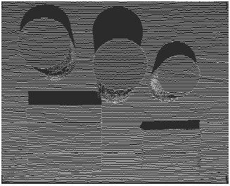
Figure 15: Laser stripes on the surface.

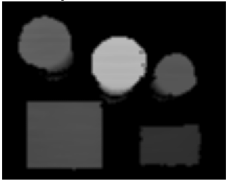
Figure 16: Perspective range image of the surface.

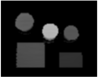
Figure 17: Orthorectified range image of the surface in top view.

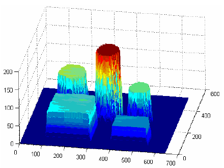
Figure 18: Orthorectified range image of the surface in 3D.

Observe the perspective effect and radial distortion in Fig. 13. The 4 crosses define the 4 fiducial marks for image plane calibration.

In Fig. 14, the surface plane is mapped in the image plane, after this, X and Y scale factors between mm and pixels have been defined.

In Fig. 16, it is clearly seen that the higher object, whose gray level is closer to white looks like bigger than it really is, as consequence of the perspective effect. In order to generate this image, bilinear interpolation has been used to fill in the unknown pixels with average values.

The Guará robot has slow movements on its 4 legs. Its speed can be set up from 450 to 800 mm/min and its step is 140 mm. The proposed system acquires and processes a new orthorectified range image when the robot stops between two steps. The processing time to obtain those images is dependable on the computer clock and camera speed which can be much lower if faster equipment is used. For the Guará robot, the processing time is suitable, allowing its navigation without compromising its performance.

V. CONCLUSIONS

By verifying the experimental results, there is no doubt about how useful these orthorectified range images are for robot navigation and control. The robots can easily find out obstacles and objects.

The rangefinder described in this paper has low cost and good precision and it is an important tool for robots. In general, the system computation time is lower and the algorithms are less complex if compared with stereo vision systems, leading to a fast acquisition and processing vision system.

Environmental light condition can vary, because this is an active triangulation system whose light source is the laser. For brighter objects, this system could be equipped with polarized lens to minimize the scattered light. For dark objects, a narrow-pass band filter could be installed on the camera lens to increase laser sensitivity or even a more powerful laser stripe could be used.

Very dark objects may absorb all laser light and no light reflection could be captured by the CCD camera. In this case, a laser profile discontinuity will occur. During the range image generation, this discontinuity is detected because of the lack of pixels. The system treats it as an unknown area of the surface. This area is avoided by the robot since it can represent a hole or an insecure place for the robot trajectory.

This system has been assembled to be used with Guará Robot, but it can be used with many other robots. As to the objects occlusion areas, while the robot walks, new images are acquired and these areas are no more occluded in the following range images. For Guará Robot, two scanning resolution have been defined: coarse scan with 35 lasers stripes, used while the robot does not find any obstacle and standard scan with 70 lasers stripes, switched when any object is found. While the former is faster, the latter is more precise.

One special feature of this system, which differs from other similar systems is the orthorectification process, which is important to correct close range image. This technique commonly used in aerial images has fit quite well for this system.

ACKNOWLEDGEMENTS
We would like to acknowledge the company Automatica Tecnologia S.A.(http://www.automatica.com.br) for helping us with personnel, equipments and facilities to make possible the realization of this work. Our sincere acknowledgements to all members of this company. We also would like to thank prof. Dr. Evandro O. T. Salles for his suggestions on this work.

REFERENCES
1. Bento Filho, A., P.F.S. Amaral, B.G.M. Pinto and L.E.M. Lima, "Uma Metodologia para a Localiza-ção Aproximada de um Robô Quadrúpede", XV Congresso Brasileiro de Automática, Gramado, Brazil (2004).         [ Links ]
2. Bertozzi, M., A. Broggi and A. Fascioli, "Vision-based intelligent vehicles: State of the art and perspectives", Robotics and Autonomous Systems, 32, 1-16 (2000).         [ Links ]
3. Everett, H.R., Sensors for Mobile Robots, Theory and Application, A.K. Peters Ltd, Massachusetts USA (1995).         [ Links ]
4. García, E. and H. Lamela, "Experimental results of a 3-D vision system for autonomous robot applications based on a low power semiconductor laser rangefinder" IEEE Proceedings of the 24^th Annual Conference of Industrial Electronics Society, 3, 1338-1341 (1998).         [ Links ]
5. Gonzalez, R.C. and R. E. Woods, Digital Image Processing, 2nd edition, Prentice Hall, New Jersey USA (1992).         [ Links ]
6. Hattori, K. and Y. Sato, "Handy Rangefinder for Active Robot Vision", IEEE International Conference on Robotics and Automation, 1423-1428 (1995).         [ Links ]
7. Haverinen, J. and J. Röning, "A 3-D Scanner Capturing Range and Color", Scandinavian Symposium on Robotics, Oulu, Finland (1999).         [ Links ]
8. Heckbert, P., "Projective Mappings for Image Warping", Image-Based Modeling and Rendering, 15-869, Beckerley, USA (1999).         [ Links ]
9. Hiura, S., A. Yamaguchi, K. Sato and S. Inokuchi, "Real-Time Object Tracking by Rotating Range Sensor", IEEE Proceedings of International Conference on Pattern Recognition, 1, 825-829 (1996).         [ Links ]
10. Qin Z., W. Li, M. Li, Z. Chen and G. Zhou, "A Methodology for True Orthorectification of Large-Scale Urban Aerial Images and Automatic Detection of Building Occlusions Using Digital Surface Maps", IEEE Proceedings of the International Geoscience and Remote Sensing Symposium, 729-731 (2003).         [ Links ]
11. Shu, F., L. Toma, W. Neddermeyer and J.Zhang, "Precise Online Camera Calibration in a Robot Navigation Vision System", IEEE Proceedings of the International Conference on Mechatronics and Automation, 1277-1282 (2005).         [ Links ]
12. Zheng, F. and B. Kong, "Calibration of Linear Structured Light System by Planar Checkerboard", IEEE Proceedings of the International Conference on Information Acquisition, 344-346 (2004).         [ Links ]

Received: December 5, 2006.
Accepted: May 22, 2007.
Recommended by Subject Editor Jorge Solsona.