ELECTRONIC NOSES APPLICATIONS AND TECHNOLOGIES

Sensors and data analysis for electronic nose

Pardo, M¹ ; Sberveglieri, G.

¹SENSOR Laboratory, Dept. of Chemistry and Physics for Engineering and Materials, University of Brescia & INFM, Via Valotti 9, I-25133, Brescia, Italy. Fax: 39 30 2091271, E-Mail: pardo@ing.unibs.it

Received November 05, 2004. In final form June 02, 2005

Abstract
The Pico Electronic Nose (EN), based on thin film semiconductor sensors, developed at the University of Brescia, is described. In particular we stress the advantages given by selecting the best features extracted from the response curves. We perform feature selection (FS) on an EN dataset composed of 30 features, obtained by extracting five diverse features from the response curves of six metal oxide sensors. We show that the performance (both classification error and PCA appearance) is always significantly better for the best features than for all thirty features. Results are not univocal regarding the best feature type. Yet, for three out of four datasets, in which the complete dataset can be decomposed, the features extracted over the sensor desorption lead to higher performances. The standard R/R₀ situates in the lower part of the ranking.

Resumen
Se describe la Nariz Electrónica Pico, basada en semiconductores de películas delgadas, desarrollada en la Universidad de Brescia. Se remarcan las ventajas que se obtienen eligiendo las mejores características extraídas de las curvas de respuesta. La selección de características se hace sobre un conjunto de datos compuesto de treinta características, obtenidas extrayendo cinco características diversas de las curvas de respuesta de seis sensores de óxidos metálicos. Se observa que el comportamiento es significativamente mejor para las mejores características que para el conjunto total de treinta. Los resultados no son unívocos respecto al tipo de la mejor característica. Sin embargo, en tres de cuatro conjuntos de datos, en los cuales el conjunto completo puede ser descompuesto, las características extraídas en la desorción del sensor conducen a mejores comportamientos. El estándar R/R₀ corresponde a la parte inferior de la clasificación

Introduction
Electronic noses (EN), in the broadest meaning, are instruments that analyze gaseous mixtures to discriminate between different (but similar) mixtures and, in the case of simple mixtures, to quantify the concentration of the constituents. ENs consist of a sampling system (for a reproducible collection of the mixture), an array of chemical sensors, electronic circuitry, and data analysis software [1].
Chemical sensors, which are at the heart of the system, can be divided into three categories according to the type of sensitive material used: inorganic crystalline materials (e.g. semiconductors, as in metal oxide semiconductor field-effect transistor structures, and metal oxides); organic materials and polymers; and biologically derived materials.
The sampling system depends on the sample type and on its preparation. For simple gas mixtures, automated gas mixing stations consisting of certified gas bottles, switches, and mass flow controllers are used. In the case of complex odors like food odors, the volatile fraction (the so-called headspace) is formed inside a vial where a certain amount of odor-emitting sample is placed.
Data analysis is a fundamental part of the EN, as it is for any sensor system or analytical instrument. This is not the case for basic research on materials for gas sensing, where the focus is traditionally the single sensors, which give higher responses or higher sensitivity (or lower detection limit) towards a single gas (possibly with minor interferents). Analysis of results is done visually, by inspecting response curves of single sensors at various concentrations. There is normally an absence of (statistical) validation.
The case of ENs is different: a step toward real-world experimental conditions is performed. What matters is the difference between responses (selectivity), not the magnitude of the responses towards single gases (sensitivity). Since single sensors are normally not selective, arrays have to be used. Analysis by inspection becomes impossible: ENs are judged (validated) by their prediction capabilities. “Enough” data have to be collected and recorded to assess prediction capabilities, and this in turn gives importance to automated measurement and recording system (production of a database) and consequently to the analysis of the data. ENs need diverse specialists.
Electronic noses have found two main application areas: food quality control and environmental monitoring. The use of ENs for food quality analysis is two-fold: to discriminate different classes of similar odor-emitting products and to predict sensorial descriptors of food quality as determined by a panel (described generically as correlating electronic noses and sensory data). Therefore, ENs can represent a valid aid for routine food analysis. The second major application area of ENs is environmental monitoring, e.g. malodours evaluation [8]. The comparative advantage in on-site landfill measurements, for example, is the big odor intensities at stake; hence, sensitivity is less of an issue. The disadvantage, on the other hand, is the difficulty in reproducible sample collection. On-site measurements are difficult because of changing environmental conditions. There is, therefore, a need for lengthy training, so that the training set is representative of all the operating conditions, or for an effective screening. Lab measurements are difficult because the sampled gas degrades rapidly.
The combination of gas chromatography (GC) and mass spectroscopy (MS) is still the most popular technique for the identification of volatile compounds [2], because the separation achieved by the GC technique is complemented by the high sensitivity of MS and its ability to identify the molecules eluting from the column on the basis of their fragmentation patterns. The main drawbacks of the approach are, however, the cost and complexity of the instrumentation and the time required to fully analyze each sample (around one hour for a complete chromatogram). Comparatively, ENs are simple and less expensive devices. They recognize a fingerprint, that is a global information, of the samples to be classified. This means that, in contrast to GC/MS, the EN does not single out and quantify each headspace component: only the global effect on the sensors is registered. Apart from GC/MS, the sensory characteristics determined by a panel are important for odor quality assessment [3]. While humans are still the most efficient instruments for sensorial evaluation, the formation of a panel of trained judges is expensive.
This article focuses on the Pico Electronic Nose system and on data analysis. The Pico EN was first designed at the Sensor Lab in Brescia and was then engineered, and is now commercialized by the SACMI Company (Imola, Italy, www.sacmi.it) as the Electronic Olfactory System EOS⁸³⁵. EOS⁸³⁵ uses advanced control electronics and has a user-friendlier data analysis interface compared to the Pico EN.
The advantages of the Pico EN are the sensor type and the data analysis software. Thin-film semiconductor sensors are stable and sensitive, while a suitably developed Matlab toolbox enables reliable analysis, even of small data sets. For example, coffee samples were classified with more than 90% accuracy with Principal Components Analysis (PCA) and Multilayer Perceptrons (MLP). More importantly, EN data were correlated with panel test judgments [4]. The Pico Electronic Nose has also been successfully tested for other applications: to discriminate extra virgin from non-extra virgin olive oil [5]; to determine the presence of bacteria and fungi in flour and maize [6]; to monitor the health of plants for manned space missions [7].

MOS Sensors and EN Measurements
Gas sensors based on the chemical sensitivity of metal oxides semiconductors (MOS) are readily available commercially and have been more widely used to make arrays for odor measurement than any other single class of gas sensors. Although many metal oxides show gas sensitivity under suitable conditions, the most widely used material is tin dioxide, SnO₂, doped with small amounts of catalytic metal additives, such as palladium or platinum. The gas is sensed by its effect on the electrical resistance of the SnO₂ semiconductor, resulting from combustion reactions occurring with lattice oxygen species on the surface of the SnO₂ particles. By changing the choice of catalyst and operating conditions, SnO₂-resistive sensors have been developed for a range of applications, for example by adding Pt we obtain a H₂S sensor [9], while the addition of Mo produces an ammonia sensor [10]; although in all cases, the resulting sensors are not highly selective and remain responsive to a large number of combustible gases. To gain the needed selectivity, several slightly different sensors (sensor arrays) and multivariate data analysis are used.
Recent trends in the sensor field concern the simultaneous measure of more than one sensor property (e.g., conductance and surface potential) or the use of different sensor types (so-called hybrid arrays) to reduce the collinearity of the responses and, therefore, obtain better discrimination.
The real challenge in the sensor field, which hampers a diffuse spread of the technique, still remain the stability of sensors over time (onset of drift) and reproducibility, both inside a single batch and from batch to batch. Since the materials are nanostructured and the working temperatures are over 200 – 300°C, the film could degrade over time, affecting sensor stability. The difference in grain distribution explains the non optimal reproducibility from batch to batch.
The typical measurement (i.e. sensor array characterization) consists of exposure of the sensors to a concentration step, that is, a change of odor concentration from zero to c (each component of the vector stands for a gas component) and back to zero again, and the recording of the subsequent change in the characteristic property of the sensor. The change of the sensor signal output with time is referred to as dynamical response; for MOS sensors, it is a conductance change. The parameters that are routinely considered to roughly describe a single sensor response to a concentration step, and which depend on the sensor type and on the gas type and concentration to be sensed (and, of course, on the measuring conditions) are:

- The variation of the sensor response between the value in air y₀ (the so-called baseline) and the steady-state (or static or equilibrium) value in gas y_s. Depending on the sensor type, various functions of y_s and y₀ are considered the standard parameters characterizing the dynamical response.
- The degree to which the sensor recovers its baseline. Complete recovery can be hampered by desorption processes that are too slow or irreversible changes of the surface constitution (poisoning).
- The response time (i.e., the time to reach steady-state conditions in gas) and the recovery time (i.e., the time to return to the baseline value). These values depend on the adsorption and desorption kinetics of the surface-gas reactions. They are defined as a fraction of the time needed to reach a steady-state value (in gas or air) or, modeling the rise and fall as simple exponentials, as the time constants of the exponentials.
Multivariate analysis of a gas mixture data is a necessary tool for analyzing sensor array data. Visual inspections of calibration curves and responses, as done for single gases, is too lenghty and not informative enough when using the sensors in realistic applications. In the case of complex mixtures, it is not interesting (nor possible) to quantify the concentrations of the huge number of single constituents (e.g., more than 700 for coffee vapors). The calibration normally consists of making repeated measurements on different but similar classes of nominally equal samples (e.g., milk) subject to different heat treatments. It is the inherent difficulty in the reproducible preparation and measurement of samples that necessitates repeated measurements.
Normally, the cluster separation on principal component analysis (PCA) score plots is used for evaluating a electronic nose performance. To further establish a functional relationship between the measurement space and the class membership, supervised methods are employed, which need a training (calibration) phase. There is a wealth of supervised learning methods. For example, chemometrics, which stems from analytical chemistry, has its own bunch of methods (e.g. PLS, SIMCA). Neural networks, and multilayer perceptrons (MLP) in particular, have been used in different application fields. MLP are a particular class of functions (polynomials are another class), which originally were developed in parallel with the study of the brain, have been shown to have nice mathematical properties, come with an effective way of adaptively changing the values of the parameters (known as error backpropagation) and, most importantly, have given good results in different application fields.
What is generally true about learning is that the more complex the space of learning functions, the easier the onset of overfitting. E.g. with a 9 order polynomial it is perfectly possible to interpolate any set of 10 points (zero error), whatever the noise level is. In fact this amounts to learning the noise in the data and not only the underlying data generator, i.e. fitting the (actual) data too much, i.e. overfitting. Various methods exist to avoid overfitting [16].
References [11], [14] are the second editions of two established textbooks on statistical learning, [12] is a tutorial on statistical learning for electrical engineers, while reference [15] is a review of data analysis for EN.

The Pico Electronic Nose
The sensors
The Pico EN (and the EOS⁸³⁵) contains six semiconductor thin-film sensors grown by sputtering on an alumina substrate. The SnO₂ type are deposited with the Rheotaxial Growth and Thermal Oxidation (RGTO) technique [9]. The RGTO technique consists of two steps:
1) During Rheotaxial Growth a metal layer is deposited by means of physical vapour deposition on a substrate held at a a temperature higher than the melting point of the metal (232 °C for tin), forming islands of melt metal.
2) In the Thermal Oxidization step a complete metal-semiconductor transformation is obtained by keeping the metallic film for ~30 hours at 600 °C in a synthetic air flow. With oxidation, agglomerates increase their volume by ~33% and therefore build interconnections allowing current flow.
The thermal oxidation step of the RGTO technique results in porous, nano-sized agglomerates and hence in stable sensors [13]. This sensor type has been tested for more than one year under different conditions, and the response stability toward a few target gases like CO and ETOH is better than ±3%.
Since the growing conditions are controllable, they can, to some degree, be tailored to a particular application. A thin layer of noble metals can subsequently be deposited as a catalyst to improve sensitivity and selectivity.
Another important parameter in the production of gas sensors is reproducibility and, for RGTO, the reproducibility of the resistance in air and gas in the same batch is better than ±2 %.
Altogether, these optimal results make the sensors unique and particularly suitable for a electronic nose, where stability and reproducibility (e.g., for transferring the training between different ENs) are important.

Data analysis
A statistical toolbox permits the classical tasks of the data analysis cycle to be performed; for these experiments, a set of Matlab functions (a toolbox) was developed [4], [15]. This set included:
- Signal preprocessing (median filter for spike removal, noise averaging) and plotting (for gaining a first impression of the response curves).
- Exploratory analysis. First, various plots of the response curves and of the features are drawn for each sensor separately (univariate analysis). After having visually checked single sensors, the complete sensor array response is checked. The most important multivariate tool for exploratory analysis is PCA (score and loading plots). PCA is implemented with a simple user interface that allows selection of the sensors and classes to be displayed, along with grouping of classes. PCA also serves for feature reduction before the use of multilayer perceptrons (MLP).
- Learning with MLP. The inputs to the MLP are the projections of the data on the first m principal components (the so-called PCA scores). The number of inputs m (PCA dimensions) is then a variable to be optimized. To prevent overfitting, early stopping or weight decay regularization can be used. Furthermore, the decomposition of the global learning tasks in successive classification subtasks [16] (hierarchical classification) has been addressed. First classification between the more distinct clusters is performed, and then the finer differences are determined in subsequent steps. This is particularly useful when dealing with a big number of classes and a small number of data.

Advanced data analysis with feature selection (FS)
Selecting good feature (sensor) subsets can help both in the understanding of the sensors themselves and in enhancing the data analysis (e.g. classification performance) through a more stable data representation. In statistical pattern recognition the phenomenon of the “curse of dimensionality” has been often observed, where the sparseness of the data in high dimensional spaces causes a bad classification performance. At the same time, two trends in sensor systems are the increase of the sensor numbers and the extraction of complex patterns from each sensor. We gave a first demonstration of the usefulness of FS for a hybrid e-nose [18].
The particular application problem investigated here is the optimal coffee ripening time. A dataset has been collected with the EOS⁸³⁵ EN from SACMI. We present here the results for one classification problem out of four we tackled (each regarding a different set of experimental conditions). In each case the classification is between four levels of post-roasting coffee seasoning. Experimental details and PCA visualizations of the data can be found elsewhere [19].
From each sensor response curve, we extracted five different features. Three are standard features: the classical R/R₀ (taking R as the minimum of the response curve during the absorption) and the integral of the response curve, calculated during the absorption (AIN) and the desorption step (DIN). We also used the approach of calculating the features in the phase-space [20]. The phase-space is spanned by the response and its first time derivative (the time variable is implicit in the trajectory described by the sensor). In this space, we calculated the integral of the trajectory during the absorption and desorption steps, named Absorption Phase Integral (APS) and Desorption Phase Integral (DPS) respectively. In Figure 1 we show the PCA plot obtained from the complete dataset, i.e. without selecting features.
To get a high classification performance and to evaluate the contribution of each feature and sensor type we performed FS. The FS selection criterion is the cross validation of the test set error for the 3 Nearest Neighbors classifier. We performed an exhaustive search over all subsets constituted by 1, 2, 3, 4, 5 features out of 30. For the 5 features sets, this means evaluating 30 pick 5 equal 75900 subsets, which required 21h of computation with a P4 processor.
Synthetically, the main result is that performance (as judged from both classification error and from PCA appearance) is always significantly better for the best features than for all 30 features. Moreover -for some of the 5 features types- performance with all 30 features is worse than performance with just the 6 features of a single type.
In Figure 2 we summarize the performances of the best feature subsets over different sets of features. The stars are the best classification ratios for FS over all 30 features. With 4 features we get the best result: almost 100%. The star symbols are always higher than the other ones. The remaining symbols represent the best classification ratios for FS inside each category of features (from the best single sensor to all 6 sensors). Inside each feature category, maximal performance is reached with 2-4 features (i.e. sensors). This means that FS is beneficial also if only one feature type is extracted.

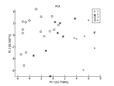
Figure 1 PCA plot for all sensors. The four symbols refer to four coffee seasoning levels.

Finally, the continuous line is the classification ratio for the 3NN over all features (no selection): it is 25% worse than the ratio for the best 4-features set. It is also worse than the performance obtained by selecting the best features from the ‘phase after’ and ‘integral after’ (‘after’ means during the desorption phase, while ‘during’ corresponds to adsorption).
For this dataset the features extracted while the gas desorbs from the sensors are better, while the standard R/R₀ has a bad performance. Yet, considering also the other three classification problems (not shown), results are not univocal regarding the best feature type. Still, for 3 out of 4 datasets the phase integral calculated on the desorption wins. Also, features (phase and integral) calculated on the desorption seem to consistently give higher performance than the corresponding features calculated during adsorption. The standard R/R₀ stands in the lower part of the ranking.

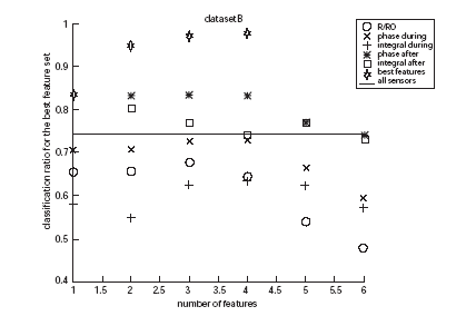
Figure 2 Best classification results for different sets of features.

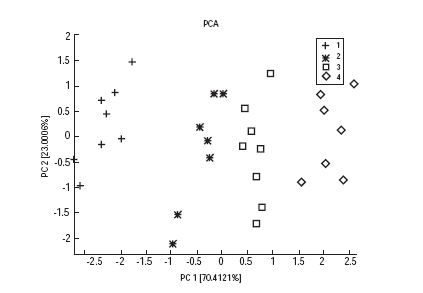
Figure 3 PCA plot for the best 4 features subset

Surprisingly, by investigating the composition of the best feature sets obtained from all features, R/R₀ plays an important role again. For example, the three highest scoring two feature sets, contain a R/R₀ feature. It seems that, while by themselves the R/R₀ features are not discriminative, they are complementary to the other features and therefore helpful for increasing performance. The advantage given by FS can also be appreciated in this case by comparing the PCA plots for all 30 features (Figure 1) and for the best 4 features (Figure 3). We see that Classes 2 and 3 are mixed in Figure 1, while they are separated in Figure 3.

Conclusions
The E-Nose Pico finds its strength in the thin film semiconductor sensors and in the data analysis software. We applied the EN to the monitoring of coffee seasoning, concentrating on the advantages given by selecting the best features extracted from the sensor responses.
We showed that simply increasing the number of features doesn’t lower the performance of a sensor system with respect to a single class of sensors/features, while a properly chosen subset does. We conclude that FS is mandatory when harvesting many features from the response curve and that it is better to use only one feature type if FS is not going to be applied.
Furthermore, FS can lead to an understanding of the data by ranking the features according to their contribution to classification. This means that, for our data, we can infer which are the best sensors and the best feature extraction methodology.

References

[1] Gardner, J.; Bartlett, P.N., Electronic Noses, Oxford University Press, 1999.         [ Links ]

[2] Mellon, F. in Spectroscopic Techniques for Food Analysis, edited by R. Wilson, Wiley-VCH, Weinheim, Germany, 1994.         [ Links ]

[3] Pal, D.; Sachdeva, S.; Singh, S., J. Food Sci. Technol. 1995, 32, 357.         [ Links ]

[4] Pardo, M.; Sberveglieri, G., IEEE Transactions on Instrumentation and Measurement, 2002, 51, 6.         [ Links ]

[5] Pardo, M.; Sberveglieri, G., Gardini, S.; Dalcanale, E., Sens. Actuators B, 2000, 69 17.         [ Links ]

[6] Falasconi, M.; Gobbi, E.; Pardo, M.; della Torre, M., Bresciani, A.; Sberveglieri, G., Sensors and Actuators B 2005, 108, 250-257.         [ Links ]

[7] Baratto, C.; Faglia, G.; Pardo, M.; Vezzoli, M.; Boarino, L.; Maffei, M.; Bossi, S.; Sberveglieri, G., Sensors and Actuators B 2005, 108, 278-284.         [ Links ]

[8] Stuetz, R.M.; Fenner, R.A.; Hall, S.J.; Stratful, I.; Loke, D., Water Sci. Technol. 2000, 41, 41.         [ Links ]

[9] Sberveglieri, G.; Groppelli, S.; Nelli, P.; Perego, C., Sensors and Actuators. B, 1993, 15 - 16 , 86 – 89.         [ Links ]

[10] Zampiceni, E.; Bontempi, E.; Sberveglieri, G.; Depero, L.,Thin Solid Films, 2002, 418 ,16-20.         [ Links ]

[11] Duda, Hart & Stork. Pattern Classification (2nd edition). John Wiley & Sons, 2001        [ Links ]

[12] Jain, Duin, Mao, Statistical pattern recognition: A review, IEEE Transactions on PAMI, 2000, 22(1), 4-37.         [ Links ]

[13] Comini, E.; Guidi, V.; Frigeri, C.; Riccò, I.; Sberveglieri, G., Sens. Actuators, B, 2002, 84, 26.         [ Links ]

[14] Webb, A., Statistical Pattern Recognition, 2nd Ed., John Wiley & Sons, Ltd. (Chichester, UK, 2002.         [ Links ]

[15] Pardo, M.; Sberveglieri, G., , Sensors Journal 2002, 2, 203.         [ Links ]

[16] Pardo, M.; Sberveglieri, G.,. Sensors Journal, 2004, 4, 3.         [ Links ]

[17] Pardo, M.; Sberveglieri, G.; Masulli, F.; Valentini, G., Anal. Chim. Acta, 2001, 446 223.         [ Links ]

[18] Pardo, M. et al., Sensors and Actuators B 2005, 106, 137-144.         [ Links ]

[19] Falasconi, M.; Pardo, M.; Sberveglieri, G.; Riccò, I.; Bresciani, A., Sens. Actuators, B 2005, 110, 73-80.         [ Links ]

[20] Martinelli, E.; Falconi, C.; D’Amico, A.; Di Natale, C., Sensor and Actuators B, 2003, 95,132.         [ Links ]