DOI: http://dx.doi.org/10.4279/PIP.100008

Physical pendulum experiment re-investigated with an accelerometer sensor

 

C. Dauphin,^1,2* F. Bouquet³

* E-mail: cyril.dauphin@villebon-charpak.fr

1 Instituí Villebon- Georges Charpak, Université Paris-Sud (Bát. 490) - Rué Héctor Berlioz - 91400 Orsay, France.
2 Département de Physique, University Paris-Sud, Université Paris-Saclay, 91405 Orsay cedex, France.
3 Laboratoire de Physique des Solides, CNRS, University Paris-Sud, Université Paris-Saclay, 91405 Orsay cedex, France.

---

We have conducted a compound pendulum experiment using Arduino and an associated two-axis accelerometer sensor as measuring device. We have shown that the use of an ac-celerometer to measure both radial and orbital accelerations of the pendulum at different positions along its axis offers the possibility of performing a more complex analysis compared to the usual analysis of the pendulum experiment. In this way, we have shown that this classical experiment can lead to an interesting and low-cost experiment in mechanics.

---

 

I.    Introduction

The physical pendulum experiment is the typical one to introduce the physics of oscillating systems. The usual aim of the analysis of this experiment is to determine the pendulum period and damping factor by using an angular position sensor [1,2].

We have conducted the pendulum experiment by using a two axis accelerometer sensor. Such sensor has already been used by Fernandes et al. (2017) [3] but their study focused on the analysis of the time variation of the radial acceleration to investigate large-angle anharmonic oscillations.

Here, we have used the accelerometer to measure both radial and orbital accelerations of the pendulum at different positions along its axis, which offers the possibility of performing a more complex analysis compared to the usual single measurement of the pendulum period.

Furthermore, we use a microcontroller and an associated two axis accelerometer sensor to acquire the data. Thus, we have used this simple and low cost experiment compared to the ready to use commercial one to introduce a richer theory and data analysis tools that can lead to an interesting experiment in mechanics.

We have described the theoretical analysis of this experiment and present an example of a possible experimental setup, the analysis of the measured radial and orbital acceleration in order to acquire the moment of inertia, the center of mass, the damping factor and the period of the pendulum.

II.    Example of experimental setup

We use an Arduino [4] and a two-axis accelerometer sensor as measuring devices. The Arduino is an in-teresting choice for an experiment, as it is an easy-to-use and low-cost microcontroller, with a large user community. Even if Arduino was not initially developed as a physicist tool, it can be used in vari-ous contexts of experimental physics activities (e.g., see references [5–10]).

 

The experimental setup that we used here is shown in Fig. l(a). The accelerometer sensor is a microelectromechanical inertial sensor which is precisely calibrated by using the valúes -\-g, Og and —g for each axis with g = 9.8 ms~².

The pendulum used in this experiment is com-posed of a bar on which masses can be attached to different positions. The accelerometer is attached to the bar and positioned in such a way that one of its measurement axes lies parallel to the bar (Fig. l(b)). Special care should be taken so that the wires connecting the accelerometer to the board are flexible enough in order not to damp the pendulum.

Figure 2 shows an example of data acquired by the accelerometer. The main features of the graph are:

•  the radial acceleration measurement decreases and goes to g as t approaches the infinity.

•  when the radial acceleration reaches its máximum valúes, the orbital acceleration is essen-tially equal to zero (inset of Fig. 2).

•  the radial acceleration is asymmetric about the straight line a = g contrary to the orbital acceleration that is symmetric about the line a = 0.

• the period of the radial acceleration oscilla-tions is twice that of the orbital acceleration oscillations (inset of Fig. 2).

In the next section, we will present the theory that explains these main features.

III.     Theory

i. Expression of the acceleration compo-nents measured by the accelerometer sensor

Applying the angular momentum theorem to the pendulum and considering viscous damping leads to:

where 9 is the angle between the pendulum axis OG and the vertical axis, M is the mass of the sys-tem and 7 is the coeflicient of friction.   We note I\ = aML² where the numerical factor a depends on the type of pendulum (a = 1 for a simple pen-dulum and a =¿ 1 for a physical pendulum). We introduce the damping factor k =

Forces acting on the proof mass (m_sensor) inside the accelerometer are its weight and the inertial forcé due to its movement. Thus, the radial and orbital components of these forces in the non-inertial reference frame of the pendulum are given by:

The acceleration components, as measured by the accelerometer at a distance r from the pivot, are then given by:

Including the expression of 9 (Eq.   (2)) into the expression of ag gives :

We choose 9 = 9q and 9 = 0 as initial conditions of the pendulum movement. We only consider here

Some comments can be made about Eqs.   (11) and (12). We first focus on the radial acceleration

•   cos(cos(x)) and sin (x) are both 7r-periodic functions. So a_r is a 4? periodic function with T = — being the pendulum period. Indeed, the pendulum reaches its máximum velocity and so its máximum radial acceleration each time 9 is equal to 0.

•   gcos (#oe~^KÍ cos(wt)) varíes between between gcos(9o) and g (blue curve in Fig. 4(b)) and goes to g as t approaches infinity. Physically, this function represents the projection of g onto the pendulum axis OG.

•   rüj¹9\e~'^ltít sin (cot) varíes between rw²#g and 0 and the upper envelope of this function (red curve in Fig. 4(b), note that it has been displaced by g) decreases exponentially as e~^2/íí. Physically, this function represents the acceleration due to the radial centrifugal forcé felt by the sensor (as expected, the acceleration due to the radial centrifugal forcé is máximum when the pendulum is vertical). This point and the previous one explains the asymmetry of the radial acceleration about the straight line a_r = g, as observed in Fig. 2.

We can now study the orbital acceleration ag:

• sin(cos(x))  and sin(x)  are both 27r-periodic functions.  Therefore, ag is a T-periodic function with T = —. Indeed, the angular ac-celeration 9 reaches its highest and lowest valúes each time the pendulum passes through its highest points. This point explains that the period of the radial acceleration is twice that of the orbital one.

•   — -j-— a sin (9ne ^Kt cosícot)) goes to 0 as t approaches infinity and the sin(cos(x)) function implies that the upper and lower envelope of this part of the ag function are symmetric about the straight line of equation a = 0 (red curve in Fig. 5(b)).

 

 

ii.     Experimentally accessible quantities

The parameters describing the pendulum and its motion can be derived from the measurements of a_r and ag.

Thus, the mea-sured valué of a_r at t = 0 leads to the valué of

•  A fit to the measured a_r upper envelope with an exponential function allows us to determine the damping factor k of the pendulum from Eqs. (11) and (12). While, for small deflection angles 6, see Eqs. (13) and (14), exponential fit of any envelope of measured a_r or ag allows us to determine the damping factor.

• The sensor position O A can be measured with great aecuracy. Thus, the position of the pendulum center of mass and moment of inertia are the two quantities which are difiicult to determine experimentally. Here, we use the fit of the temporal evolution of a_r and ag to determine the product o.L.

iii.     Impact of a and r on the measured radial and orbital accelerations

Figure 7 displays the evolution of the radial and orbital accelerations with time for different valúes of the moment of inertia (from a = í (Panel (a)) to a = 2.5 (Panel (d))). At the difference of the radial acceleration, we can see that the orbital acceleration depends strongly on a. Indeed, ag expression at í = 0 leads to ag(t = 0) = (-V — 1) gsin#₀, which is an inverse function of a. We can also note that aglt = 0) < 0 if a > -f and aglt = 0) > 0 if a < -7-. Thus, valué of ag at t = 0 gives infbrmation on the a valué.

Figure 8 shows the evolution of the radial and orbital accelerations with time for different valúes of r. The distance OA increases from Panel (a) to Panel (d). As expected, the amplitude of the radial acceleration increases with larger O A valúes as the centrifugal forcé acting on the proof mass increases and the amplitude of the orbital acceleration decreases with larger O A valúes as the rate of variation of 9 decreases with this distance.

In particular, acceleration components measured by the accelerometer attached to the position of the point O are given by:

In this case, the only forcé acting on the mass inside the accelerometer is its weight and the expressions of the acceleration do not depend on a. Accelerometer sensor is used in this case as an angular position sensor.

We also note that the acceleration components measured by the accelerometer attached to the position r = La are given by:

In this case, component of 9 due to the gravity forcé is counterbalanced by the orbital component of the forcé of gravity acting on the accelerometer sensor. Thus, ag is then directly proportional to the pendulum angular velocity.

After having shown that Eqs. (11) and (12) ex-plain the features observed experimentally we will now use them to retrieve the pendulum parameters k, a and L for different experimental setups.

IV.     Example of data analysis

i.     Example with a pendulum bar

We first focus on the pendulum shown in Fig. 9 to derive its physical parameters. We use a bar of a 45 cm length and mass 45 g with the pivot at 16.5 cm from the center of mass and the accelerometer at 33 cm.

Figure 10 shows the radial and orbital accelera-tions measured by the accelerometer after the pendulum has been displaced from the equilibrium po-sition to an initial angle of 22°.

We have analyzed the data using Eqs. (11) and (12) with k and a as free parameters. The results of the fit are shown as black curves in Fig. 10. We have derived the best fit for l/n = 12.2 s and a = 1.56.

Assuming the pendulum to be a simple homoge-neous slab, we calcúlate that the inertia moment of the bar about the rotation axis A is equal to 1.93 x 10~³kgm², which leads to a = 1.62. The holes in the bar, which are used for attaching the masses, together with the mass of the accelerometer, explain the difierence between this and with the a valué obtained from the data fit. This exper-iment allows us to determine with a good accuracy the moment of inertia of the pendulum.

 

ii.     Retrieval of the mass center position

The pendulum of the previous subsection is a sym-metric bar, thus, its mass center position can be determined precisely. In the general case, the mass center position can be difiicult to determine and we can fit the data by using Eqs. (11) and (12) with k, a and L as free parameters and infer the position of the center of mass.

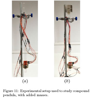
As an example of such analysis, we use a pendulum composed of a bar on which several masses can be attached to at different positions to acquired data that corresponds to pendulums of different valúes of a and L (Fig. 11 (a) and (b)).

Figure 12 (a) and (b) displays the radial and orbital accelerations measured by the accelerometer after each pendulum shown in Fig. 11 has been displaced by an initial angle of 20.5°.

We fit the data by using Eqs. (11) and (12) with k, a and L as free parameters. Results of the fit are shown as the black curves in the insets of Fig. 12. Best fit are obtained with Í/k = 111 s, a = 1.162 and L = 0.293m for the pendulum of Fig. ll(a) and Í/k = 101 s, a = 6.55 and L = 0.074 m for the pendulum of Fig. ll(b).

For the examples displayed in Fig. 12, the evo-lution of the orbital acceleration from Panels (a) to (b) shows an increase of a, which is consistent with the fact that pendulum configuration goes from a configuration cióse to a simple pendulum (a ~ 1 Fig. ll(a)) to a compound pendulum (a > 1 Fig. 11(b)).

Figure 12 shows that the angular acceleration (in green) is much more sensitive to the valué of a than the radial acceleration (in red). Therefore, orbital acceleration is a good quantity to measure and to fit in order to determine the moment of inertia of a pendulum.

iii.     Impact of r on the acquired data

We have shown in section III that the orbital acceleration is very sensitive to the accelerometer sensor position with respect to the pendulum rotation axis. As this position is precisely known, we can perform several measurements with different positions of the accelerometer to improve the accuracy and/or the precisión of the derived pendulum parameters. As an example of such analysis, we use the experimental setups shown in Fig. 13.

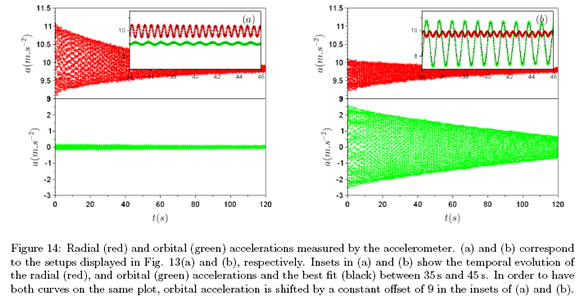
Figure 14 (a) and (b) display the radial and orbital accelerations measured by the accelerometer after each pendulum shown in Fig. 13 has been displaced by an initial angle of 20.5°.

Fits of the data using Eqs. (11) and (12) with k, a and L as free parameters are shown as black curves in Fig. 14. Best fit are obtained with Í/k = 111 s, a = 1.162 and L = 29.3 cm for the pendulum of Fig. 13(a) and with Í/k = lOOs, a = 1.162 and L = 29.2 cm for the pendulum of Fig. 13(b).

The position of the accelerometer does not af-fect the calculated valúes of the moment of inertia of the pendulum and only slightly affects the cen-ter of mass position. The new configuration of the wires connecting the accelerometer in Fig. 13(b) changes slightly the k valué. Thus, performing a second measurement with a different position of the accelerometer allow us to be more confident in the results retrieved from the first one.

We can also note that the orbital acceleration increases with lower O A valúes, therefore the orbital acceleration fit precisión is better when the accelerometer is in the position of Fig. 13(b), while the precisión of the radial acceleration fit is better when the accelerometer is in the position of Fig. 13(a).

V.     Conclusions

We have shown that the pendulum experiment ana-lyzed with an accelerometer sensor leads to a theoretical study richer than the classical one. We have derived theoretical expressions for the radial and orbital acceleration data recorded by an accelerometer and separated the contributions from the pendulum angular motion and the gravitational force on the proof mass.

We have also shown that the orbital acceleration is an interesting data to retrieve the moment of inertia of a pendulum.

The possibility to have different positions of the sensor allows us to perform several measurements with the same pendulum to improve the accuracy and/or the precision of the derived pendulum pa-rameters.

In this paper, we have only focused on the clas-sical pendulum but the device used here could also be applied to more complex systems such as chaotic pendulums.

 

Acknowledgements - This work benefited from a grant "P´edagogie innovante" from IDEX Paris-Saclay. The Institut Villebon - Georges Charpak was awarded the Initiative of Excellence in Inno-vative Training in March 2012 (IDEFI IVICA: 11-IDFI-002), and is supported by the Paris-Saclay Initiative of Excellence (IDEX Paris-Saclay: 11-IDEX-0003). The authors would like to thank the referee for his/her helpful comments.

[1]  http://www2.vernier.com/sample_labs/ PHYS-AM-18-physical_pendulum.pdf

[2]  https://physics.fullerton.edu/files/ Labs/225/Physical_Pendulum_V4_l(1).pdf

[3] J C Fernandes, P J Sebastiáo, L N Goncalves, A Ferraz, Study of large-angle anharmonic os-cillations of a physical pendulum using an ac-celeration sensor, Eur. J. Phys. 38, 2017.

[4]  https://www.arduino.cc

[5] S Kubínová, J Slégr, Physics demonstrations with the Arduino board, Phys. Educ. 50, 472 (2015).

[6] C Galeriu, S Edwards, G Esper, An Arduino investigation of simple harmonio mo-tion, Phys. Teach. 52, 157 (2014).

[7] K Atkin, Construction of a simple low-cost tes-lameter and its use with Arduino and Maker-Plot software, Phys. Educ. 51, 024001 (2016).

[8] C Petry et al., Project teaching beyond Physics: Integrating Arduino to the laboratory, In Technologies Applied to Electronics Teach-ing (TAEE), pp. 1-6, IEEE (2016).

[9] R Henaff et al., A study of kinetic friction: The Timoshenko oscillator, Am. J. Phys. 86, 174 (2018).

[10] F Bouquet, J Bobroff, M Fuchs-Gallezot, L Maurines, Project-based physics labs using low-cost open-source hardware, Am. J. Phys. 85, 216 (2017).