Inglês (pdf)
 Artigo em XML
 Referências do artigo
 Enviar este artigo por email
 Citado por SciELO
  Similares em
SciELO
Similares em
SciELO 
 Permalink
INTRODUCTION
Violence is one of the main challenges in Brazil in the last three decades. This phenomenon imposes huge costs on society, estimated at around 5% of GDP every year. In 2010, when the last census was conducted in Brazil, homicides were already escalating rapidly throughout the country. This census invalidated a logic hitherto assumed to be true: the largest states and metropolitan regions would be responsible for the highest number of murders in the country. Actually, three smaller states were pointed as the ranking leaders.
According to data from the Mortality Information System (SIM) of the Ministry of Health (Brasil, 2019), Alagoas was in first place, with 66.8 cases per 100 000 inhabitants, followed by Espírito Santo (50.1), and Pará (45.9).
Although several articles have explored this theme for other states in Brazil (Sartoris, 2000; Almeida, Haddad & Hewings, 2005; Lima, Ximenes, Souza, Luna & Albuquerque, 2005; Pereira & Queiroz, 2016; Gomes, Evangelista, Lima & Parré, 2017; Sass, Porsse & da Silva, 2016), we chose Alagoas, since it lead the homicide ranking per 100 thousand inhabitants in 2010, at the time of the national census.
Alagoas is in the northeast and is the second smallest state in Brazil (Figure 1). However, it has the highest population density in the country. Besides being a poor region, in the last decade the state was classified as one of the most violent, raising its rate until 2014 and then decreasing it in the following four years.
Furthermore, the main Brazilian criminal organization, which emerged in São Paulo’s prisons, has recently expanded its activities to other Brazilian states. This expansion was initially driven unintentionally by the penitentiary system itself, which, in order to isolate the organization’s leaders, exiled them to different prisons around the country.
This resulted in adverse side effects, increasing the organization’s geographical influence (Manso & Dias, 2018).

Financed with major robberies and trafficking resources, the organization advanced across the country, especially in the northeast state capitals, clashing with local criminal groups and traffickers for territory. These disputes raised the homicide rate in the metropolitan regions of the northeast capitals, which include Maceió, capital of Alagoas. Therefore, these rates in Brazil increased considerably. Even inside the prisons, the confrontations were brutal, provoking several rebellions with a significant number of deaths. At the same time, violent regions like São Paulo and Rio de Janeiro saw a reduction in the proportion of homicides in the country’s total (Manso & Dias, 2018).
Using data from the last available census (2010) for education, income, wealth concentration, population, and other variables linked to the crime economics theory, we applied a cross-section spatial model in order to eliminate spatial autocorrelation and observe the social impact on homicides. Therefore, this paper aimed to verify the influence of socioeconomic variables on the homicide rate in the municipalities of Alagoas. This was done by adjusting the estimation due to the existence of verified spatial autocorrelation, that is, the presence of neighbor spillover effects.
The first part of the article contains a brief literature review focused on the crime theory, space and crime and some empirical experiences. Our first analyses are based on the exploratory spatial data analysis (ESDA) methodology. This has been widely used in the last twenty years, highlighting Messner, Anselin, Baller, Hawkins, Deane and Tolnay (1999), who developed a work about the spatial patterning of county homicide rates in a particular region of the United States. This methodology provides data, methodological considerations and tools employed, as the Moran’s Index for global analysis, and the LISA method, to detect autocorrelation of municipal homicides rates and homicides clusters in Alagoas, as well as results and analysis. Thus, a spatial model was chosen and applied in order to fix the spatial correlation, and new parameters were established to explain the impacts of several socio-economic variables on homicide rates. The results show a significant influence of poverty on homicide rates.
I. CRIME, SPACE, AND SOCIETY
Brazil faces a serious structural problem of violence. The emergence of criminal organizations, militias, and the trafficking war in poor communities in big cities has substantially risen murders in many regions over the past 20 years. Violence has recently become an increasingly important issue in developing countries. The mainstream literature always tries to capture the incentives that would be taken into account in a criminal’s decision making through microeconomic concepts, in other words, the individual’s choice between living an ordinary life, or trying the criminal one.
Incentives are almost always based on two sets of results. The first set would be the benefits of the crime, such as wealth or other desired reward. The second one would be the negative factors, such as the likelihood of arrest, conviction, death, or other collateral damage, in addition to moral, ethical, and psychological elements. This set of variables would guide, usually informally, individual decisions.
Economic studies related to crime have gained greater visibility from Gary Becker’s article entitled “Crime and Punishment: An Economic Approach “(1968), considered a milestone in this field. The author used economic theory to understand the determinants of crime, emphasizing the relationship between costs and benefits, crime and punishment. Becker’s model is based on rationality, where individuals weigh their actions in relation to legality or illegality, seeking profit and analyzing the probabilities of being caught and the punishments applied (Becker, 1968).
Ehrlich (1973) was the first researcher to develop a theoretical model to explain criminal behavior, in which individuals face a work/leisure trade-off by allocating work time to legal or illegal activities. Therefore, offenders would respond to the same type of incentives as people in legal activities, even after being arrested. Furthermore, his work shows a positive relationship between income inequality for all variety of crimes and the opposite for the arrest probability (Ehrlich, 1973).
Several economists and other social scientists use economic theory and econometrics to measure the factors that determine crime, in this case the homicide rate. Such attention in Brazil is fully justified by the fact that this rate has almost doubled in the last twenty years. In the northeast of the country (NE), where the most violent cities are concentrated, crime has become a chronic problem.
According to the Atlas of Violence 2019 (Cerqueira, 2019), in 2016 the country’s average was 30.3 homicides per hundred thousand inhabitants and, in the NE, it was 44.15. This indicator is used to analyze and compare the crime level between cities in many countries, since homicides are considered the most serious acts of violence and it is also easy to obtain reliable data. In this paper, we brought together economic and demographic variables to help explain crime in space. Some studies led by economists and sociologists have shown that demographic factors are crucial in defining the propensity for criminal life.
Bronfenbrenner (1979) argued that the environment influences individual development in many ways. At each stage of the moral development process of individuals, relationships in different contexts will lead to right and wrong references, determining whether there will be a moral cost for committing a crime. Conceição, Scorzafave and Costa (2021) indicated that the development of individuals depends on their interaction with the environment in which they are involved. Becoming more inclined to commit or suffer violence is also part of this interaction.
Regarding crime and its relationship with the size of cities, Glaeser and Sacerdote (1999) stated that crime rates are higher in large cities, because the probability of identification and arrest after a crime is lower due to the population size. Therefore, individuals have higher expected returns from crime in large cities. In addition, studies on crime show better results when conducted in smaller geographic units than those that seek to analyze it internationally.
In the Brazilian literature, we found several crime studies in different knowledge fields, such as anthropology, psychology, sociology, and economics, among others. Concerning the latter field, econometric models are usually employed in order to identify the impact of each socioeconomic determinant on crime rates. The main reference is Becker’s model (1968), but the lack of equivalent data worldwide to replicate empirical studies makes it very difficult to use.
Even so, some studies have been conducted, such as in Rio de Janeiro (Zaluar, 1985), and in Minas Gerais, in which Beato Filho (1998) showed the importance of socioeconomic variables in explaining crime. Other articles provide empirical evidence on the relationship between Becker’s socioeconomic variables and homicides, such as income, inequality in education, return to crime, probability of punishment, and weighing of city sizes (Cerqueira & Lobão, 2003; Oliveira, 2005). In many cases, the data point to crime spatial patterns and spillover effects. Thus, it is necessary to adopt an econometric approach different from the ordinary one, the spatial econometrics, which comprises the impact measuring on these variables influenced by neighbors in space.
Using this approach in Minas Gerais and based on census data (1991), Beato Filho (1998) found a strong spatial concentration of property crime in larger cities. The authors indicated that the murders, however, often occurred in places lacking infrastructure, especially basic sanitation.
In Brazil, research has been conducted for specific regions, measuring the influence of socioeconomic variables on crime, controlling for space. For São Paulo, Sartoris (2000) and Rodrigues (2005); in Rio de Janeiro, Szwarcwald and Castilho (1998); for Pernambuco, Lima et al. (2005); in Sergipe, Jorge (2013); and for the state of Paraná, Sass et al. (2016). Castro, Silva, Assunção and Beato Filho (2004) analyzed the spatial distribution of homicides in Minas Gerais, from 1996 to 2000, and found 24 spatial conglomerates with similar homicide rates. This result allowed developing a policy called Public Security Management Units.
Using data from 1999-2001, Carvalho, Cerqueira, and Lobão (2005) conducted a homicide rate mapping for municipalities in Brazil in order to capture any spatial patterns. The main conclusion was that there is homicide concentration in the metropolitan regions. Given the rising numbers and the scarcity of studies on crime in the northeast, especially in Alagoas, it is interesting to verify the occurrence of spatial effects, as well as to determine its direction, positive or negative, characterized by violent regions side by side with areas of low rates (Cooter & Ulen, 2007).
Therefore, this study aimed to analyze the causes of homicides in the municipalities of Alagoas, based on socioeconomic variables, controlling for spatial correlation through a spatial model. Economic variables can explain a considerable part of the variation in the homicide rate among municipalities. Other demographic indicators such as population, percentage of poor people, and unemployment are used in the model to better study homicides. The objective of this article was to identify the influence of socioeconomic variables on homicides.
II. DATABASE AND METHODOLOGY
A common problem when estimating crime impacts is the strong correlation and multicollinearity that many explanatory variables have. Although this does not affect the quality of the estimator, it is difficult to obtain significant estimators for these important variables indicated by the theoretical models. The homicide rate per 100 000 inhabitants is the chosen dependent variable, according to the International Classification of Diseases (ICD-10). Homicide deaths per household (X85 to Y09) were gathered from the SIM by the DATASUS source for the year 2010.
Socioeconomic data were collected from the 2010 IBGE Census and homicide information, from the SIM for Alagoas municipalities. Homicide in Brazil is eminently a male, black, and young phenomenon. The relationship between age and crime in the working-age population is clearly established in the literature. The probability of committing a crime increases from the age of 15 and drops sharply from the age of 29, reaching a peak between the ages of 15 and 24 (Blumstein, Cohen, Roth & Visher, 1986; Herrnstein & Wilson, 1998).
The variables “municipal population” and “population density” were included to test the criminals’ agglomeration tendency in major cities. Probably, such agglomeration can occur for two reasons. First, the larger the population, the more difficult it is to capture the criminal. Second, it should be easier to find tools for crime, since the available weapon and explosive supply tends to be greater in larger cities.
Police force data were also gathered from the 2010 IBGE Census, including Federal Police Officers, Federal Highway Police, Municipal Guard, and Legislative Officers by municipality. This variable was chosen to help measure the dissuasive effect across municipalities.
Crime and the unemployment rate tend to have the same sign. Thus, the unemployment rate of people 16 years and older was adopted. Studies indicate that schooling changes the opportunity cost of criminal activity, as the more years of education people complete, the higher their wages and employment opportunities, which implies a greater cost of crime for more educated agents (Becker, 1968). Lochner (2020) stated that school attendance keeps individuals busy and, consequently, off the streets, reducing the possibility of early entry into criminal activities.
The relationship between inequality, poverty, economic development, and violence can be considered one of the most controversial explanation lines. Although there are many studies on this subject, the results are often divergent. In order to facilitate the results interpretation, we transformed some variables, such as population, which was divided by 1000, and the Gini index, which was expressed as deviations around the mean. We excluded other variables after performing a correlation test, since they indicated the presence of severe multicollinearity problems. Among the correlated variables, we selected those with greater variability in order to obtain a better model, including all the desired dimensions according to the theoretical support.
III. EXPLORATORY SPATIAL DATA ANALYSIS - ESDA
One of the most widely disseminated methods to verify spatial autocorrelation is the Moran statistic, where the null hypothesis refers to spatial randomness (Messner et al., 1999). Carvalho and Albuquerque (2011) argued that this test can be applied to the variable yi directly or to yi residual regression versus a set of explanatory variables. Thus, it is considered a linear regression model:
 (1)
(1)
Where y is a column vector (n x 1) of response variables; X is a matrix with each row comprising the observations for the explanatory variables and a unitary column associated with the intercept of the model; β is a coefficient vector; and u is a column vector with the regression residuals. From now on, we used the estimate of ordinary least squares for the coefficient vector, obtaining the expression for the residuals as follows:
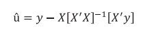 (2)
(2)
Therefore, we have our variable of interest (y) and its spatial lag (Wy), which is standardized with mean zero and variance equal to 1, transforming into z. Thus, to calculate Moran’s I, we considered the following simple linear regression:
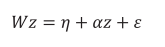 (3)
(3)
The calculation of Moran’s I is equivalent to estimating the slope coefficient of Equation (3).
This index ranges from -1 to 1, providing a measure of linear association between the Ut
vectors and the weighted average of the neighborhood values (WZt
). As it has an expected value of
However, global autocorrelation can omit statistically significant behavior patterns at the local level, which is why local spatial autocorrelation indexes have been created with the ability to identify differentiated spatial association regimes. The most widely used of these is the Local Moran’s Index described by the following equation:
 (4)
(4)
Then, if Local Moran’s I > 0, there is an indication of clusters with similar values around i; if Moran’s I < 0, this implies clusters with different values around i; when Moran’s I = 0, it evidences that there are no clusters (Silva, Borges & Parré, 2013).
Firstly, to analyze the neighbors, we created a first-order Queen-type weight matrix, which was found to be better suited to data. Figure 2 shows the histogram of the first-order Queen matrix with the number of neighbors and frequency (between 2 and 11 neighbors).
According to Anselin (1996), the Moran scatter plot is one of the ways to interpret this statistic. Otherwise, it is a representation of the regression coefficient that allows visualizing the linear correlation between z (normalized variable) and Wz (average of neighbors) through the graph of two variables. Thus, the Moran’s I coefficient represents the slope of the Wz regression curve against z, which indicates the degree of adjustment (Figure 3).
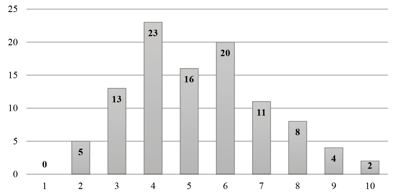
Source: prepared by the authors in Geoda software.
Figure 2. Histogram of the number of neighbors and frequency in the municipalities of Alagoas
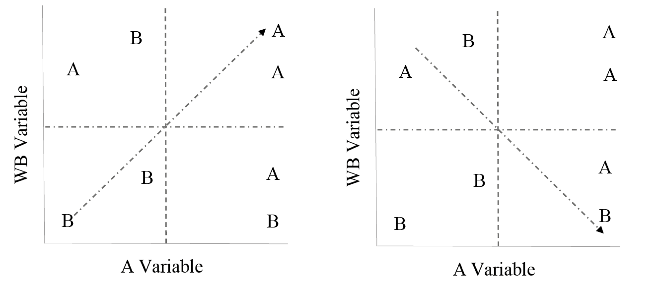
This diagram is divided into four quadrants. The first one, (Q1), contains the regions that present high values for the variable under analysis surrounded by regions that show values above the mean for the analyzed variable. Q1 is called High-High (AA). The second quadrant (Q2) includes the regions with low values surrounded by neighbors that present high values; classified as low-high (BA). In the third quadrant (Q3), there are regions with low values surrounded by neighbors that also have low values; called low-low (BB). Finally, the fourth quadrant (Q4) comprises regions with high values surrounded by neighbors with low values; classified as high-low (AB) (Perobelli, Almeida, Alvim & Ferreira, 2003).
Regions found in Q1 and Q3 denote points with positive spatial autocorrelation, that is, such regions form clusters of values. Therefore, regions located in Q2 and Q4 present a negative autocorrelation. Figure 4 illustrates the scatter plot resulting from the distribution of the variable test of the homicide rate. Thus, based on the measured slope, we can affirm that there are clusters of high-high and low-low values in Alagoas municipalities.

Source: prepared by the authors in Geoda software.
Figure 4. Moran’s Index - Homicide rate in Alagoas in 2010
Monteiro, Câmara, Carvalho and Druck (2004) emphasized that, after calculating the Moran’s Index, it is necessary to validate it. Such validation can be performed through the pseudo-significance test, where up to 999 permutations of different values associated with attributes with the regions are generated. Each one produces a new spatial arrangement where the values are distributed. The implicit hypothesis of the calculation of the Moran’s Index is that the data are stationary in first and second order.
If the originally measured Moran’s I value corresponds to one extreme of the simulated distribution, it is statistically significant. Hence, we performed 999 permutations to identify whether or not to reject the autocorrelation hypothesis. The positive and significant Moran statistic result points to spatial dependence in the homicide rate of the municipalities of Alagoas according to Figure 5.
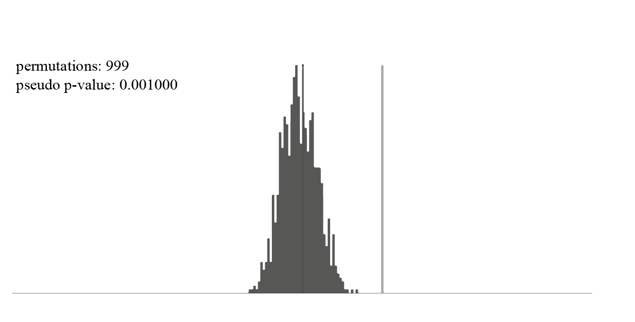
With this result, the null hypothesis of randomness cannot be accepted and, consequently, two situations may be possible: a) municipalities with high homicide rates would be geographically close to each other, or b) municipalities with low homicide rates would be surrounded by others with low homicide rates. However, the presence of both clusters and significant spatial outliers may be hidden and therefore not captured by a single global indicator. Hence, the local Moran’s test was used. This test is a thematic map that resulted in a non-random behavior of the homicide rate in the municipalities of Alagoas.
For this purpose, we used the LISA (Local Indicator of Spatial Analysis) tool, which provides, for each observation, an indication of the existence of spatially (statistically) significant clusters of similar values around that observation (Figure 6).
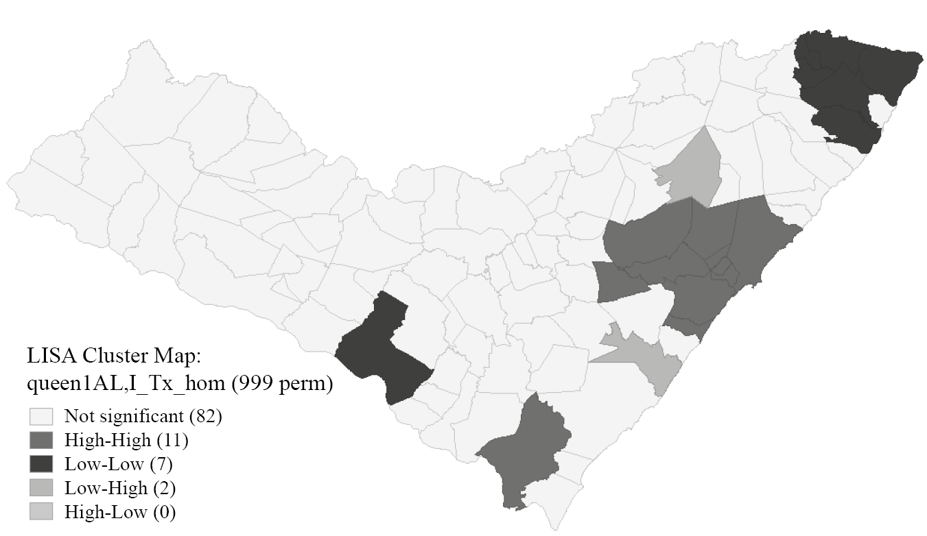
The previous result shows that most municipalities (78.43%) are not clustered by homicide rates. These are represented in gray. Thus, these localities do not have a standardized behavior in their respective homicide rates at the significance level considered. Most of the significant municipalities are on the outskirts of Maceió (21.57%), the capital city. This region and the municipality of Penedo have been identified as having high homicide rates and are also surrounded by others with this characteristic.
Among the significant data, 27.3% refers to the municipalities that are in blue. These represent the low-low type interaction, that is, localities with low homicide rates surrounded by others with similar homicide rates. Based on LISA results, we can see signs of local spatial autocorrelation. Thus, both global and local aspects indicate that the homicide rate in Alagoas has spatial spillovers.
IV. THE SPATIAL MODEL
Besides Moran’s I and LISA, our work applied spatial econometrics, since traditional models cannot control spatial autocorrelation caused by the spillovers that the variables produce on and receive from their neighboring ones. Another situation that can be corrected by spatial econometrics is the correlation between errors, which can also be due to territory heterogeneity.
To perform the regression, we used the socioeconomic database of the municipalities of Alagoas, extracted from the 2010 IBGE Census and other databases. The homicide rate was the dependent variable, for the year 2010, extracted from the SIM. The sample comprises 102 municipalities of Alagoas. The variable homicide rate was chosen because it is the most reliable and realistic crime statistic available in Brazil. Across the country, crime statistics such as robberies, thefts, rapes, etc. are inaccurate and often undercounted. A national information system on public security is still under development and lacks historical series. Homicide data, on the other hand, are far more reliable, as they are registered and provided mandatorily by the Ministry of Health. An analysis aggregating other types of crime, such as robberies, burglaries, or thefts, would introduce additional bias in the results.
The police registration frequency varies from crime to crime and from place to place, depending on the population’s trust in law enforcement, as well as factors such as having insurance coverage or not, the victim’s relationship with the aggressor, the amount of money involved, and previous experience with the police. In addition, many events can be resolved in an “amicable” manner, through conflict mediation even by the police force. Thus, these may not be filed in formal police reports ( Jorge & Prates, 2021). There are estimates that this underreporting is around 80% in Brazil (Viapiana, 2006, p. 137).
Table 1 describes the socioeconomic variables used to explain the homicide rate behavior, the database sources, some of the principal papers in the literature that used them, and the expected sign of these variables according to the crime economics literature.
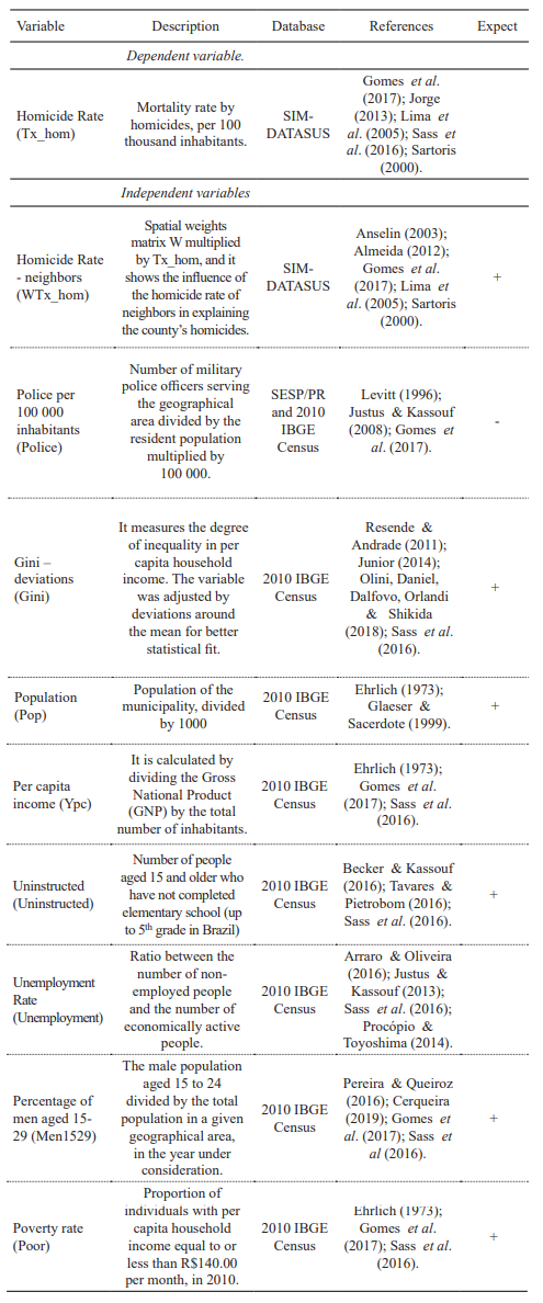
Table A1 in the Appendix shows the descriptive statistics of the same variables. Our main results are based on the Queen spatial weight matrix “W”, which was chosen to verify horizontal, vertical, and diagonal interactions. Later, we demonstrate some further analysis founded on an inverse distance matrix.
But first, it was necessary to choose the model to use in the study. Thus, we had to estimate the classical model (MQO). Afterwards, based on this first estimation, it was possible to define the choice of the best option for the model.
The estimated regression is represented as follows:
 (5)
(5)
The ordinary least squares estimation method was performed to indicate the most appropriate model, thus verifying the incidence of spatial autocorrelation operating on the survey data. Lagrange Tests, also known as score tests, are based on the first-order optimization approach of the Lagrange function in the logarithmic probability function represented by:
 (6)
(6)
Where n is the Lagrange multipliers vector, which is equivalent to q restrictions in
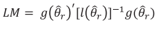 (7)
(7)
Whereis
It should be noticed that the result obtained (Moran’s I = 0.1451) points to signs of spatial autocorrelation. Therefore, MQO was inappropriate to address the spatial dependence problem. Thus, the most appropriate model was the one that did not present any evidence of spatial autocorrelation on its residuals.
Since spatial autocorrelation was detected, we could not estimate the model with ordinary least squares, and we needed to choose a suitable model controlling for spatial dependence. Therefore, we assessed the model through the OLS (Table 2) only to get an indication about where the spatial dependence was located, and which was the best model to apply.
Table 2 . Output Ordinary Least Squares

Source: own elaboration based on research data with GeoDa software.
We verified the results of the Lagrange Multiplier LAG and Error tests and their respective robustness in Table 3.
Table 3 . Spatial dependence and Lagrange Multiplier Tests
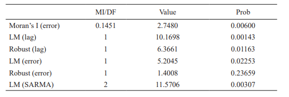
Source: own elaboration based on research data with GeoDa software.
Thus, as can be seen, the most appropriate model to use in this case was the spatial LAG, since the Error model was not significant for spatial correlation. The spatial autoregressive model (known as SAR or Lag model) is one of the most applied for spatial correlation modeling. Its characteristic is that it uses the same idea of autoregressive models in time series, by incorporating a Lag term (Carvalho & Albuquerque, 2011).
The biggest difference is that the spatial Lag does not refer to the same variable in the past, but to the same variable in the neighbors. Therefore, in this case, it is not a temporal analysis, but a simultaneous one. Anselin (2003) stated that, in the Spatial Lag Model, the previously ignored autocorrelation is attributed to the dependent variable Y. Thus, the addition of a new term to the regression model is considered as a spatial relationship. In its simplest form, the SAR model has its expression written as follows:
 (8)
(8)
Where y is a column vector; n is the number of observations in the sample for the response variable yi; Xβ represents the set of explanatory variables and the beta parameter; p is the scalar coefficient that corresponds to the autoregressive parameter, which is interpreted as the dependent variable average effect, referring to the spatial neighborhood of the region (the Alagoas state). On the other hand, it is equivalent to a column vector containing residuals from the equation.
Despite the advantages in controlling for spatial effects in the applied models, we must highlight a limitation regarding endogeneity. In this case, it may occur due to the omission of important variables or because of reverse causality, which is the case of the variable Police, where localities with worse homicide rate indicators are expected to have greater coverage of police services.
Some studies such as the one by Di Tella and Schargrodsky (2004) sought to control for the causal effects of the Police Force, but, unfortunately, we did not have available data for applying strategies that address this causal inference. Therefore, the effects should be interpreted with caution.
The Jarque-Bera test has as null normality hypothesis (JARQUE & BERA, 1987). Thus, if p > 0.05, normality is not rejected. In our study, with this statistic resulting in p = 0.31357, the sample errors have a normal distribution. The Jarque-Bera test shows that the errors distribution is normal. Hence, it could be estimated by the Maximum Likelihood. However, this is an asymptotic test, and 102 observations is too small a sample to be reliable and considered as asymptotic1.
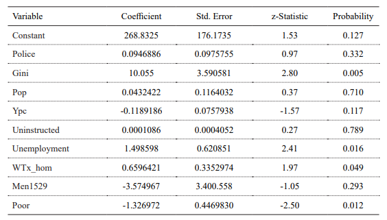
Using the GeoDa Space software, we estimated the regression applying the GMM method in spatial two stage least squares (S2SLS). Thus, Table 4 details the results obtained.
Table 4. Spatial Lag estimation with GMM in Spatial Two Stage Least Squares (S2SLS)

Source: own elaboration based on research data with GeoDa Space software.
Again, Lag W was highly significant, at 1%, showing the neighboring influence impact on the homicide rate of 0.60. In addition, the Anselin-Kelejian spatial diagnostic test confirmed that the spatiality problem was fixed. The results suggest interactions in the space captured by the spatial Lag model. Besides being affected by neighbors, the homicide rate was influenced by the variables income concentration (Gini), Unemployment, and Poor, the only one with inverted sign, regarding the theory. The effect of spatial lag on the homicide rate was also significant at 5%.
Unemployment has followed the economic intuition, and it showed that increasing this rate has a positive impact on the homicide one. Although the theory does not reveal a direct relationship between unemployment and crime, which means that it cannot be demonstrated that unemployed individuals tend to commit crimes, we have there a specific situation that can contribute to the understanding of Alagoas.
It is known that the most frequent victims of homicides are young people between 15 and 29 years old, men, black, and who live in the poorest communities of large cities. Precisely this population group is the most affected in the first place by unemployment and greater vulnerability due to lack of opportunities (Perobelli et al., 2003).
In addition, research on crime in Brazil indicates the movement of criminal organizations such as the First Command of the Capital (PCC, as per its initials in Portuguese) to the north and northeast markets over the last decade, where Alagoas is located ( Manso & Dias, 2018). The employability jeopardized even by their individual address together with the possibility of high returns from drug trafficking may lead young people who are included in this situation to opt for a life that increases the possibility of being victimized. Hence, in this case, there might be a relationship between unemployment and homicides.
The Gini index was statistically significant at 5%, corroborating the theory and indicating that the greater the income concentration, the greater the homicide rate. Regarding the variables Ypc, Police, Pop, Men1529, and Uninstructed, we could not draw any conclusions, since they were not significant for this analysis. Although the variable Uninstructed was not significant, Grogger (1998) argued that the greatest impact of education is through its role in determining income, and not directly through a reduction in crime propensity.
One caveat should be made: the fact that these variables are not significant does not imply that they are not necessary for the best model adjustment, since removing these variables, or just one, would cause important changes, and all of them are strongly related to the theory.
In order to verify how sensitive our results were to the spatial weight matrix choice, we did some tests, as shown in Table A2 (Appendix), where the inverse distance matrix was used. As can be seen, the main conclusions were maintained, the variables of income inequality and unemployment rate have a statistically significant effect and increases in these variables are related to higher homicide rates in Alagoas. In addition, the variable Poor again presents the opposite impact to that expected. The effect of spatial lag on the homicide rate was also significant at 5%.
On Table A3 (Appendix), we sought another test of the robustness of our results by including the variable proportion of black individuals in our base model. Again, the main conclusions were maintained, either qualitatively or even in terms of magnitude. The variable race was not significant. A possible explanation is that, although we expected this factor to be important in terms of individual data, when we aggregated for the relationship of the municipalities of Alagoas, the expected link disappears. This is because, in this case, we would be analyzing differences between the aggregated units, no longer in individual terms, and greater homogeneity may occur. A similar fact must be true for the variable Men1529.
In the same way, Table A4 (Appendix) shows the SAR model estimation by the GS2SLS estimator, using both Queen and the inverse distance matrix. The estimation presents direct and indirect effects with each spatial weights matrix. Results reveal that the significant effects of the variables Gini, Unemployment, and Poor occur via direct effects, and indirect spillover effects were not statistically significant.
CONCLUSION
In 2010, according to the violence map, Alagoas was the leading state in Brazil in homicide rate with the terrible mark of 66.8 homicides per 100 000 inhabitants. Among the state capitals, Maceió appeared as the most violent: 109.9 homicides per 100 000 inhabitants. This study provided some knowledge about this problem, through an impact analysis between the homicide rate and socioeconomic data, also understanding the reciprocal influence among municipalities.
The empirical model used in this study presented the results expected by the theoretical model, reaffirming the ability of economics not only to contribute to the explanation of the homicide rate, but also to suggest more efficient public policies. The most important conclusions reached in this analysis refer to income concentration and unemployment. In cities where income concentration increases, so do homicides. The unemployment rate greatly affects the one of homicides. An increase in unemployment is reflected in the homicide rate.
Socioeconomic indicators, such as unemployment rates and income distribution, showed that crime can be the result of worse economic conditions, and not just a simple choice between gains and losses. In this view, crime must be explained by a wide range of disciplines from many fields, not just economics. Violent crime in a region can only be effectively prevented through investments in urbanization, professional training, state infrastructure, public services, and police presence (Menezes, Silveira Neto, Monteiro & Ratton, 2021).
This study has some limitations related to endogeneity as discussed earlier, a small number of observations due to the number of municipalities, and potentially less heterogeneity among municipal indicators in Alagoas.