


Serviços Personalizados
Journal

Artigo
 Inglês (pdf)
 Artigo em XML
 Referências do artigo
 Enviar este artigo por email
Indicadores
-
 Citado por SciELO
Links relacionados
-
 Similares em
SciELO
Similares em
SciELO
Compartilhar

 Permalink
Revista de la Unión Matemática Argentina
versão impressa ISSN 0041-6932versão On-line ISSN 1669-9637
Rev. Unión Mat. Argent. v.46 n.2 Bahía Blanca jul./dez. 2005
Principal eigenvalues for periodic parabolic Steklov problems with L∞ weight function
T. Godoy, E. Lami Dozo and S. Paczka
Partially supported by Fundacion Antorchas, Agencia Cordoba Ciencia, Secyt-UNC, Secyt UBA and Conicet
Abstract: In this paper we give sufficient conditions for the existence of a positive principal eigenvalue for a periodic parabolic Steklov problem with a measurable and essentially bounded weight function. For this principal eigenvalue its uniqueness, simplicity and monotone dependence on the weight are stated. A related maximum principle with weight is also given.
2000 Mathematics Subject Classification. 35K20, 35P05, 35B10, 35B50
Let  be a
be a  and bounded domain in
  with
with  and
and  let
let  and let
  ,
,  be two families of real functions defined on
  and
and  respectively, satisfying for
  that
that  and
and  are
are  periodic in

![∂aij (-- ) ∂xi ∣[0,T] ∈ C Ω × ℝ](/img/revistas/ruma/v46n2/2a0517x.png) and
and  Let
Let  be a nonnegative and
  periodic function belonging to
  for some
  Assume in addition that for some
  and for all

(1)
where 
 and
and  Let
Let  and let
  be the
  matrix whose
  entry is
  Assume also that
  is uniformly elliptic on
 ![-- Ω × [0,T]](/img/revistas/ruma/v46n2/2a0536x.png) , i.e., that there exists a positive constant
, i.e., that there exists a positive constant  such that
(3)
for all  ,
,  Let
Let  be the periodic parabolic operator defined by
(4)
where  denotes the standard inner product on
  . Finally, let
  be a nonnegative and
  periodic function in
  and let
  be the unit exterior normal to
  Under the above hypothesis and notations (that we assume from now on) we consider, for a
  periodic function (that may changes sign)
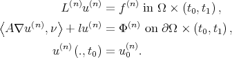
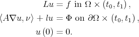
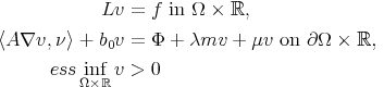
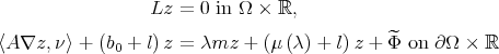
  the periodic parabolic Steklov principal eigenvalue problem with weight function
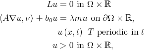
(5)
the solutions understood in the sense of the definition 2.1 below. In order to describe our results let us introduce, for  the quantities
(6)
In this paper we prove (cf. Theorem 6.1) that if either  and
and  or
or  and
and  and if
  (respectively
  ) then there exists a positive (resp. negative) principal eigenvalue for (5), that is, a
  whose associated eigenfunction
  satisfies (5). Under an additional assumption on
  a similar existence result is also given for the case
 .
.
Our approach, adapted from [4] and [8], reads as follows: If we change  in (5) by
  we have the following one parameter eigenvalue problem: given
  find
find  such that this modified (5) has a solution. We prove in section 4 that this problem has a unique solution
  which satisfies that
  is real analytic and concave. We also obtain an expression for
  which allows us to decide the sign of
  In section 5 we prove that
  (respectively
  ) implie
  (resp.
  ). From these facts, and since the zeroes of the function
  are exactly the principal eigenvalues for (5), our results will follow.
Sections 2 and 3 have a preliminar character. In section 2 we collect some general facts about initial value parabolic problems and in section 3 we study existence and uniqueness of periodic solutions for parabolic problems and we prove some compactness and positivity properties of the corresponding solutions operators related.
Let us start introducing the notations to be used along the paper. For a topological vector space  we put
  for its topological dual and
  for the corresponding evaluation bilinear map
  If
If 
 are normed spaces and if
  is a bounded linear map we denote by
  (or simply by
  if no confusion arises) its corresponding operator norm. If
  is a real Banach,
  and
and  we put
  for the space of the measurable functions (in the Bochner sense)
  such that
  We define also
  and, for
  the space
  , similarly (with the obvious changes) to the corresponding usual Lebesgue's spaces. For
  we put
  for the space of the
  periodic functions
 satisfying that
  We write also
  (respectively
  ) for the space of the
  periodic functions belonging to
  (resp. to
  ). The spaces

 and
and  equipped with their respective norms

![-- ∥∥C(Ω)×[0,T]](/img/revistas/ruma/v46n2/2a05115x.png) and
and ![∥∥C(∂Ω)×[0,T]](/img/revistas/ruma/v46n2/2a05116x.png) are Banach spaces. For
are Banach spaces. For  we will identify (writing
  ) the spaces
and also the corresponding spaces of functions defined on 
Let  be the real Hilbert spaces
 equipped with their usual norms. For
  let
let  be the space of the indefinitely differentiable Frechet functions from
  into
into  ,
,  equipped with the topology of the uniform convergence on each compact subset of
  of the function and all its derivatives. Let
  be its dual space. For
  let
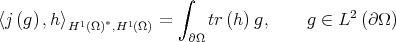
let  be its distributional derivative defined by
  for all
  where
where  denotes the inner product in
  We will say that
  if there exists a function (denoted by
  ) belonging to
  such that
  for all
For  let
let  be the bilinear form defined by
(the values on ![∫ aL,b0 (t,g, h) = ∫ [〈A (.,t)∇g, ∇h 〉 + 〈b(.,t),∇g 〉h + a0 (.,t)gh] + b0(.,t) gh Ω ∂Ω](/img/revistas/ruma/v46n2/2a05144x.png)
(7) of
of  and
and  understood in the trace sense) and let
  be the bounded linear operator defined by
(8)

 and
and  let
let  be defined by
 and
and 
for some positive constant depending only on 
 and
and  We set also
(11)
and  So
So  equipped with the norm
  is a Banach space. With these notations we can formulate the following definition
Definition 2.1. For 
 ,
,  and
and  we say that
 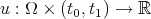 is a solution of the problem
(12)
if  and
and  a.e.
a.e. 
¿From now on, a solution of a boundary problem like (12) (except if otherwise is explicitely stated) will mean a solution in the above sense.
Remark 2.2. For 

 with
with  standard computations on the quadratic form
  give, for all
and also
where  is the ellipticity constant of
  So, for
  and
and  there exists a positive constant
  depending only on
  and
and  such that
(13)
for all  and
and  Moreover, for such
  and
and  the assumptions on the coefficients of
  imply that there exists a positive constant
  such that
(14)

for all  and
and 
For  as in Remark 2.2,
 and
and  consider the problem
(16)
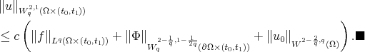
Note that ![W τ,t ⊂ C ([τ,t],X)](/img/revistas/ruma/v46n2/2a05205x.png) (cf. ([12], Lemma 5.5.1) and so the initial condition
(cf. ([12], Lemma 5.5.1) and so the initial condition  makes sense. Taking into account the facts in Remark 2.2, ( [12], Theorem 5.5.1) applies to see that (16) has a unique solution
  Let
Let  be the linear operator defined by
Let us recall the following properties (cf. [12], Theorem 5.4.1) of the evolution operators 
Remark 2.3. i) Given  with
with  there exists a positive constant
  such that, for
(17)
ii) Since  (the isomorphism
  given by duality) we can consider
  In this setting, it holds that for
  as above there exists a positive constant
  such that
(18)
for  and
and  Since
Since  (and then also
  ) is dense in
  it follows that
  has a unique bounded extension to an operator (still denoted
  ) from
  into
into  which satisfies, for
  as in (18),
(19)
Finally, we recall also that for  it holds that
(20)
For  ,
, and
and  consider the problem
(21)
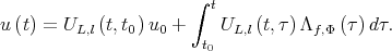
Taking into account (13), (14) and (15), ([12], Theorem 5.5.1) applies to see that (21) has a unique solution  given by
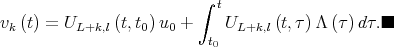
(22)
Remark 2.4. Observe that  is a solution of the problem
(23)
 solves
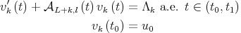
with  defined by
  . Thus (23) has a unique solution
  given by
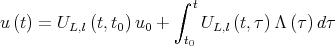
(25)
 defined by
Moreover, for ![t ∈ [t ,t ] 0 1](/img/revistas/ruma/v46n2/2a05251x.png) we have (cf. [12], Lemma 5.5.2)
we have (cf. [12], Lemma 5.5.2) 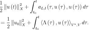
(27)
¿From (27), standard computations show that there exists a positive constant  independent of
  and
and  such that
(28)
Remark 2.5. The estimates (17), (18), (19) and (20) still hold (with another constants) for the operators  given by (26) and
  satisfies
(29)
for 
Remark 2.6. For 

 and
and  the problem
(30)
has a unique solution which satisfies in addition that

(31)
for some positive constant  independent of
 and
and  Indeed, the solutions of (30) are those of (23) taking there
  and Remark 2.4 applies.
Remark 2.7. It is easy to check that the constant  in (28) and so also in Remark 2.5 and Remark 2.6 can be chosen depending only on


 and on an upper bound of
Lemma 2.8. Let 

 and
and  be as in Lemma 2.4 and let
  be a sequence of operators of the form

with 
 and
and  satisfying for each
  the conditions stated for
  at the introduction with the same
 and
and  given there for
  Assume also that for each
  and
and 
 and
and  converge uniformly on
  to
to  and
and  respectively and that
  converges to
  in
in  . Let
. Let  and
and  be sequences in
  and in
  respectively and assume that they converge to
  and
and  in their respective spaces. Let
  be a sequence in
  that converges to
  in
in  and let
  Thus the solution
  of the problem
converges in the  norm to the solution
  of (30).
Proof. For  as in Remark 2.2,
  ,
,  and
and  , let
, let  be the solution of
and let  be the solution of (24). We have
(32)
Our assumptions imply that  and that
  uniformly on
 ![t ∈ [t0,t1].](/img/revistas/ruma/v46n2/2a05331x.png) From Remarks 2.6 and 2.7 we have that
From Remarks 2.6 and 2.7 we have that  is a bounded sequence. Then from (33)
  Thus from Remark 2.6 applied to (32) we obtain
  Since
Since  and
and  the lemma follows.
Lemma 2.9. Assume that  and
and  are nonnegative. Then the solution
  of (30) is nonnegative.
Proof. We pick sequences 

 and
and  as in Lemma 2.8 satisfying in addition that

 and such that

 and
and  belong to
 ![∞ (-- ) C Ω × [t0,t1] ,](/img/revistas/ruma/v46n2/2a05352x.png)
 belongs to
 ![C ∞ (∂Ω × [t0,t1])](/img/revistas/ruma/v46n2/2a05354x.png) and
and  Let
Let  be as in the proof of Lemma 2.8. Thus
  (cf. e.g., Theorem 5.3 in [9], p. 320)). The classical maximum principle gives
  and since by Lemma 2.8
  in
in  we get
  Since the solution
  of (30) is given by
  the lemma follows
Remark 2.10. Let us recall some well known facts concerning Sobolev spaces (see e.g. [9], Lemma 3.3, p 80 Lemma 3.4, p. 82)
i): For  and
and  with
with  we have
  and the restriction map (in the trace sense)
  is continuous from
  into
into 

ii) For  with
with  it holds that
  for
for ![t ∈ [t ,t ] 0 1](/img/revistas/ruma/v46n2/2a05376x.png) and for such
and for such  there exists a positive constant
  independent of
  such that
iii) For  the following facts hold:
![W 2,1 (Ω × (t,t )) ⊂ C1+ σ,1+2σ (Ω-× [t,t ]) q 0 1 0 1](/img/revistas/ruma/v46n2/2a05382x.png) for some
for some  with continuous inclusion.
![2- 1,1- 1 1+σ W q q 2q(∂Ω × (t0,t1)) ⊂ C1+ σ, 2 (∂ Ω × [t0,t1])](/img/revistas/ruma/v46n2/2a05384x.png) for some
for some  and with continuous inclusion.
iv) For  let
let  be defined by
  if
if  and
and  if
if  Thus
Thus  if
if  and
and  for all
  if
if  in both cases with continuous inclusion
Remark 2.11. For  it holds that
  continuously for some
  In this case, for
  , let
, let  be the space of the functions
  that satisfy (in the pointwise sense)
  where
where 
(34)
Let us recall that for such  and for
 and
and  there exists a unique
 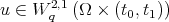 satisfying almost everywhere
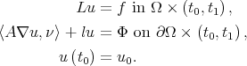
(for a proof, see [9], Theorem 9.1, p. 341, concerning the Dirichlet problem and its extension, to our boundary conditions, indicated there (at the end of chapter 4, paragraph 9, p. 351). Moreover, there exists a positive constant  independent of
  and
and  such that
Lemma 2.12. i) For 
 is a compact and positive operator.
ii) Let 
 with
with  For
For 
 and
and  the restriction of
  to
to  belongs to
  and there exists a positive constant
  such that
  for all
iii)  for
for  and
and  and
and  is a bounded operator from
  into
into 
iv) For  it hold that
  and
and  is a bounded operator from
  into
into  Moreover, if
 and
and  then
then 
v) For  and
and 
 is a compact and strongly positive operator
Proof. By Lemma 2.9  is a positive operator. It is also compact because
  is continuous (cf. Remark 2.5) and
  has compact inclusion in
  Thus (i) holds.
To see (ii) we pick a strictly increasing sequence of positive numbers  such that
  for all
  and we pick also a sequence of functions
  in
in  satisfying
  for
for 
 for
for  Let
Let  and let
  and
and  be the sequences of functions on
  inductively defined by
 and by
 respectively
 Then, for all
(35)
Let  be defined by
  and by
  (with
(with  as in (iv) of Remark 2.10) and let
  For the rest of the proof
  will denote a positive constant independent of
  non necessarily the same at each occurrence (even in a same chain of inequalities). We claim that for

(36)
with their respective norms bounded by  .
.
If (36) holds, for  Remark 2.10 (iv) gives
  Taking into account that
  on
on  Remark 2.11 gives
and so (ii) holds.
To prove the claim we proceed inductively. Since  satisfies 29, Remark 2.6 gives
  and so
  Then, by Remark 2.11,
  and so
  Since
Since  on
on  and
and  we get also that
  Thus (36) holds for
  Suppose that it holds for some
  Then
Then
 on
on  )
) 
Since  it follows that
  and so, from (35), a similar estimate holds for
  This complete the proof of the claim.
The imbedding theorems for Sobolev spaces and (ii) imply (iii). The first part of (iv) is again obtained applying (ii) with  To see the second part of (iv), we observe that if
  and
and  then
then  and, by Lemma 2.9,
  Let
Let  and
and  be as in the proof of (ii), Since
 ![2,1 1+σ,1+σ v1 = φ1u ∈ W q (Ω × (t0,t1)) ⊂ C 2 (Ω × [t0,t1]) ,](/img/revistas/ruma/v46n2/2a05514x.png) the boundary condition for
the boundary condition for  holds in the pointwise sense. Now, the Hopf parabolic maximum principle applied to
jointly with the fact that  on
on  gives (iv).
To see (v), let 
 and let
  Since
Since  (with
(with  given by (34)), from (ii) we can consider the bounded operator
  defined by
  Since the operator
  is continuous from
  into
into  and the inclusion map
  is compact, we obtain the compactness assertion of (v). Finally, the strong positivity in (v) follows from (iv).
Lemma 2.13. i) If  and
and  then
then  for
for 
ii) If  and
and  are nonnegative functions and if either
  or
or  then
then
Proof. Let 
 ,
,  be the positive cones in
 and
and  respectively and let
  be the closure of
  in
in  Observe that if
  then
then  . Indeed, if not, the Hann Banach Theorem gives
  such that
  and
and  For
For  let
let  be defined by
  Thus
Thus  for all
  Since
Since  is reflexive there exists
  such that
  for all
  In particular we have
  for all
  This implies that
  and so
  which contradicts
  Thus
Thus 
Let  so
so  and then there exists a sequence
  of nonnegative functions in
  that converges to
  in
in  Since
Since  is continuous and, by Lemma 2.12 (i), it is a positive operator on
  we have
  and so (i) holds.
To see (ii), observe that  and so (i) gives
(38)
is the solution of the problem
Then, by (i),  in
in  and since
  (because either
  or
or  ) we conclude that for some
  the set

has positive measure. Then, since  , Lemma 2.12 (iv) gives
  for all
  Now (ii) follows from (38) and (39).
Remark 2.14. Let us recall the following version of the Krein Rutman Theorem for Banach lattices and one of its corollaries (for a proof, see e.g., [5], Theorem 12.3 and Corollary 12.4)
i) Let  be a Banach lattice with cone positive
  and let
  be a bounded, compact, positive and irreducible linear operator. Then
  has a positive spectral radius
  which is an algebraically simple eigenvalue of
  and
and  The associated eigenspaces are spanned by a quasi interior eigenvector and a strictly positive eigenfunctional respectively. Moreover,
  is the only eigenvalue of
  having a positive eigenvector.
ii) For  and
and  as above and for a positive
  the equation
  has a unique positive solution if
  no positive solution if
  and no solution at all if
  In particular this implies that if
  for some positive
  then
then 
We recall also that a point  is a quasi interior point if and only if
  and the order interval
 ![[0,a]](/img/revistas/ruma/v46n2/2a05614x.png) is total (i.e. the linear span of
is total (i.e. the linear span of ![[0,a]](/img/revistas/ruma/v46n2/2a05615x.png) is dense in
is dense in  ) and that for a measure space
  equipped with a positive measure
  on
on  and
and  the quasi interior points in
  are the functions that are strictly positive almost everywhere. Moreover, for such
  a bounded and positive linear operator
  satisfying that

 for all
  is an irreducible operator (cf [13], Proposition 3, p. 409).
Lemma 2.15. For  and
and 
 is a positive irreducible operator and its spectral radius
  satisfies
Proof. By (i) and (iv) of Lemma 2.12,  is a positive, irreducible and compact operator. Thus, by the Krein Rutman Theorem,
  is positive and that is the unique eigenvalue with positive eigenfunctions associated. Moreover, by Lemma 2.10 (iii), these eigenfunctions belong to
  for
for  . Take
  By Lemma 2.12 (v),
  is a compact and strongly positive operator which, by the Krein Rutman Theorem, has a positive spectral radius
  Since the eigenfunctions of
  belong to
  we have
  Thus, to prove the lemma, it is enough to see that
We proceed by contradiction. Suppose  , let
, let  be a positive eigenfunction with eigenvalue
  and let
  . Since
 By Lemma 2.12 (ii),
  and since
  the maximum principle gives that either
  is a constant or
 ![max -- w (x, t) Ω ×[δ,T ]](/img/revistas/ruma/v46n2/2a05654x.png) is achieved at some point
is achieved at some point  If
If  is a constant, since
  the boundary condition (which is satisfied in the pointwise sense because
  ) implies
  which is impossible and if the maximum is achieved at some point
  we would have
  in contradiction with the boundary condition.
 be the Banach space
with norm 
Lemma 3.1. For 
 and
and  the problem
has a unique solution 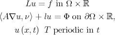
(41) .
.
Proof. Let  For
For  the solution of
is given by 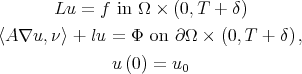
(42) 
(43)
By Lemma 2.15,  has a bounded inverse. From (25),
  if and only if
(44)
then there exists a unique solution  of
of  in
in 
 on
on  and
and  . For such a
  and for
 ![t ∈ [0,T + δ],](/img/revistas/ruma/v46n2/2a05685x.png) let
let  Thus
Thus  in
in 
 on
on  and
and  Then
Then  (i.e.,
  ) for
) for ![[0,T + δ].](/img/revistas/ruma/v46n2/2a05694x.png) Thus
Thus  can be extended to a solution of (41) which is unique by (44).
Let  be the trace operator on
  and for
  let
let  be the trace operator defined by
For  we define the linear operators
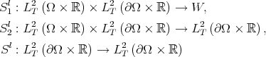
by
 where
where  is the solution of (41) given by Lemma 3.1,
respectively.
Remark 3.2. Let 
 and
and  be Banach spaces,
  and
and  reflexive. let
  be a compact and linear map and
  an injective bounded linear operator. For
  finite and

is a Banach space under the norm  A variant of an Aubin-Lions ´s theorem (for a proof see [10], p. 57 or Lemma 3 in [6]) asserts that if
  is bounded then the set
  is precompact in
We will apply this result to 
 and
and  The map
  is the trace map,
  is defined by
and  Hence
Hence  above is a special case of
  in (11) for
  which is naturally isometric to the space
  of (40).
Lemma 3.3. i) For 
 and
and  are bounded linear operators and
  is also compact
ii) If  and
and  are nonnegative and if either
  or
or  then
then  and
and  Moreover, if
  then
then 
iii)  is a bounded, positive, irreducible and compact operator on
Proof. For  and
and  the
the  periodic solution of (42) is given by (43) with
  given by (44). Remark 2.6 gives

So, to see that  is a bounded operator, it is enough to obtain see that
(45)
(for the rest of the proof  will denote a positive constant independent of
  and
and  non necessarily the same at each occurrence, even in a same chain of inequalities). Let
  Thus
Thus  solves
  in
in 
 on
on  and
and  Since
Since

(27) (applied to this problem and used with  and
and  ) gives
the last inequality by Remark 2.6. So


By Lemma 2.5,  has a bounded inverse, and so (44) and (46) give (45). Then
  is bounded and this implies the boundedness, first of
  and then of
To see that  and
and  are compact, we consider a bounded sequence
  Then, from Remark 3.2
  is bounded in
  so
so  has a convergent subsequence in
  From
From  we have that
  is also compact.
Suppose now that either  or
or  and let
  be given by (44). For
  Lemma 2.13 (iv) gives
  for
for  and, by Lemma 2.12 (ii), we have
  Then
Then  has a positive minimum
  on
on ![-- Ω × [δ,T + δ].](/img/revistas/ruma/v46n2/2a05795x.png) Now,
Now,

for ![t ∈ [δ,T + δ]](/img/revistas/ruma/v46n2/2a05797x.png) and so, by periodicity,
and so, by periodicity,  Since
Since 
 and
and  we get that
  and also that
  Then (ii) holds and
  is irreducible.
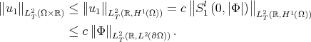
Lemma 3.4.  .
.
Proof. For  consider
  and let
  Let
Let 
 with
with 
 Thus
Thus 
 and
and 
Along the proof  will denote a positive constant independent of
  and
and  (non necessarily the same even in a same chain of inequalities). Since
  in
in  ,
,  and
and  is
is  periodic, Remark 2.6 gives
  So
So
and a similar estimate hold for  and then also for
  Now,
Now,  solves
  in
in 
 on
on  and
and  is
is  periodic. Then, from (27) used with
  and
and  we get
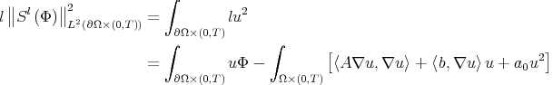
(47)
Now
the last inequality by Remark 2.6. Lemma 3.3 (iii) and Remark 2.6 give also ![∫ - [〈A ∇u, ∇u 〉+ 〈b,∇u〉 u+ a u2] Ω×(0,T) 0 ∫ 〈 ( 1 ) 1 〉 ∫ [〈 1 〉 ] = - A ∇u + -A -1b ,∇u + -A- 1b + --A-1b,b - a0 u2 Ω×(0,T) ∥〈 2 〉∥ 2 Ω×(0,T) 4 ∥ 1 -1 ∥ ∫ 2 2 ≤ ∥∥ 4A b,b ∥∥ ∞ u ≤ c ∥Φ∥L2T (ℝ× ∂Ω) . L (Ω×(0,T)) Ω×(0,T )](/img/revistas/ruma/v46n2/2a05839x.png)
(48)

Thus 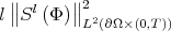
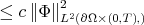 and the lemma holds.
We will use the multiplication operator  given by
(49)
For  and
and  let us observe that
  satisfies
(in the sense of the definition 2.1) if and only if for each 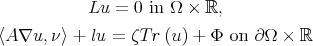
(50) it satisfies
  in
in 
 on
on  , i.e., we can "add"
  to both sides in the boundary condition of (50).
Lemma 3.5. i) For each  there exists
  such that for
  and
and  such that
  the problem (50) has a unique solution
  for all
  Moreover, it satisfies
  if
if 
ii) For such 
 and
and  the solution operator
  is a bounded linear operator from
  into
into  whose norm is uniformly bounded on
  for
for 
Proof. Let  such that
  By Lemma 3.4 there exists
 such that
  for
for  For
For  we have
  and so
  has a bounded inverse. If
  solves (50), it solves
  in
in 
 on
on  and so

|
 | (51) |
Thus the solution of (50), if exists, is unique and given by (51).
To prove existence, consider the function  defined by (51). It solves
and so 
(52) 
(53)
Then (52) can be rewritten as
and so 
 solves (50).
Suppose now  By (ii) and (iii) of Lemma 3.3,
  and
and  are positive operators and also
  Thus (51) gives
  and so (i) holds. Finally, from (51) and since
  and
and  are bounded and
  and
and  we obtain (ii).
We will need to introduce two news operators. For 

 let
let 
(54)
be defined by  where
where  is the solution of (50) given by Lemma 3.5 and by
  respectively.
Corollary 3.6. For 
 and
and  as in Lemma 3.5,
  is a bounded, compact, positive and irreducible operator.
Proof. By (53) we have

and the corollary follows from Lemma 3.3 (iv) .
.
4. A one parameter eigenvalue problem
Lemma 4.1. i) For  and
and  there exists a unique
  such that the problem
has a positive solution. Moreover, for 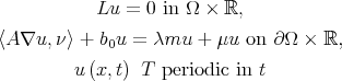
(55) positive and large enough let
  be the spectral radius of
  It holds that
 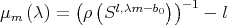 (where
  is the spectral radius of
  ).
).
ii) The solution space for this problem is one dimensional and for  positive and large enough
 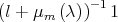 is an algebraically simple eigenvalue of
iii) Each positive solution  of (55) satisfies
Proof. Let 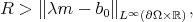 let
let  be as in Lemma 3.5 and for
  let
let  be the spectral radius of
  . From Lemma 3.6
  is a compact, positive and irreducible operator on
  Then, by the Krein Rutman theorem,
  is a positive eigenvalue of
  with a positive eigenfunction
  associated. Let
  Thus
Thus  is a
is a  periodic solution of
  in
in 
 on
on  . It is also positive because, by Lemma 3.5,
  is a positive operator. Since
  it follows that
  solves (55) for
On the other hand, if  is a positive solution of (55) then
  in
in  and
and  on
on  . So, for
 From Corollary 3.6 and the Krein Rutman theorem it follows that
  and so
  Thus (55) has a positive solution if and only if
  In particular, this gives that
  does not depend on the choice of
  and
and  . If
. If  is another positive solution of (55), for
  and as above, and since
  and
and  is an eigenfunction of
  with eigenvalue
  the Krein Rutman theorem gives
  for some
  . Thus
then the solution space for (55) is one dimensional. Again by the Krein Rutmnan theorem,  is an algebraically simple eigenvalue of
  .
.
Finally, each positive solution  of (55) satisfies

and so Lemma 3.5 (iii) gives 
The aim of the rest of this section is to given some properties of the function 
 defined, for
  , by Lemma 4.1. Each zero of
  provides a principal eigenvalue with weight
  and the corresponding solutions
  in (55) are the respective positive eigenfunctions. We will prove that the map
  is strictly decreasing in
  (Lemma 4.6) and continuous for the
  convergence in
  (Lemma 4.7) hence continuous in
 is concave and analytic in
  (cf. Corollary 4.9 and Remark 4.11).
Remark 4.2. For  let
let  be the space of the
  periodic functions on
  whose restriction to
  belongs to
  and for
  let
let  be the space of the
  periodic functions on
  belonging to
  .
.
We recall that if
 ,
,  for
for 

for such a  , then (cf. Remark 3.1 in [8]) the solutions
  of (55) belong to
  and so
  for some
  Thus Theorem 2.5 in [8] gives
In order to make explicit the dependence on 
 and
and  we will write sometimes
  or
or  for the function
Lemma 4.3. Let  and suppose that
  satisfies
(56)
for some  ,
,  and
and  If
If  and
and  then
then  If in addition either
  or
or  then
then 
Proof. If  and
and  then, by Lemma 4.1,
  Assume that either
  or
or  Since
Since  for all
  , it suffices to prove the lemma in the case
  For
For  let
let  be as in Lemma 3.5 and let
  . Let
. Let  and let
  Thus
Thus 
 and, since
 So also
  Now,
Now,

If  since
since  we have
  If
If  then (by Lemma 4.3)
  and so
  Then
Then  and thus, from (57),
  Then
Then  Also, from (57),

Let  be the spectral radius of
  Remark 2.14 (ii) gives
  and so
Lemma 4.4. Suppose  satisfies
(58)
for some  ,
,  and
and  If
If  and
and  then
then  If in addition either
  or
or  then
then 
Proof. Consider first the case when  and
and  For
For  let
let  be as in Lemma 3.5 and let
  Let
Let  be the
  periodic solution of
  in
in  ,
,  on
on  and let
  be the
  periodic solution of
  in
in  ,
,  on
on  . Thus
  and, by Lemma 3.3 (iv),
  Then
Then  and so also
  Let
Let

Since  is
is  periodic and
 Thus
Thus 
If  then
then  and so
  where
where  is the spectral radius of
  Thus, Remark 2.14 (ii) gives
 and so
  Then, by Lemma 3.3 (iii),
  This implies
  in contradiction with the assumption
  Thus
Thus 
Assume now that either  or
or  and that
  If
If  then
then  and so
  and
and  This implies
  and if
  the same conclusion is obtained. So, in both cases, (59) gives now
  in contradiction with Remark 2.14, (ii).
Since for  we have
  the case
  and
and  arbitrary follows from the previous one and, finally, the case
  follows from the case
  by considering the identity
Let  be the operator defined by
  We have
Corollary 4.5. i) Suppose  Then
Then  for all
ii) Suppose  Then
Then  for all
Proof. let  be the solution of (55). Thus
(60)
If  since
since  we have
  then Lemma 4.4 gives (i). If
  then
then  Since
Since
(ii) follows again from Lemma 4.4.
Lemma 4.6. For 
 with
with  imply
imply  for all
  and
and  for all
  .
.
Proof. Suppose  and
and  Let
Let  be a positive and
  periodic solution of
Since  on
on  and
and  Lemma 4.4 applies to give
  which contradicts our assumption
  The case
  follows from the case
  using that
  .
.
Lemma 4.7. Let  be a bounded sequence in
  which converges
  to
to  in
in  . Then
  for each
  .
.
Proof. To prove the lemma it suffices to show that for each  as in the statement of the lemma there exists a subsequence
  such that
Let  be a positive number such that
  for all
  and let
  Thus, by Corollary 4.5,
(61)
Let  be the positive
  periodic solution of
(62)
normalized by  We observe that
  is a bounded sequence in
  and so, by Lemma 3.3 (i),
  is bounded in
  Thus
Thus  is bounded in
  and
and  is bounded in
  where
where  and
and  are the linear maps defined in Remark 3.2 Then there exists a subsequence
  that converges in
  to some
  From (61), after pass to a furthermore subsequence, we can assume also that
  for some
  Thus
Thus  converges in
  to
to  Since
Since  and
and  is continuous we obtain that
  converges in
  to
to  It follows that
  i.e., that
  is a
is a  periodic solution of
  in
in 
 in
in  . Since
  and
and  converges in
  to
to  and since
  we get
  Then
Then 
Corollary 4.8. For each  the map
  is continuous from
  .
.
Corollary 4.9.  is a concave function.
Proof. Choose a sequence  in
in  that converges
  to
to  in
in  and such that
  for all
  By ([8], lemma 3.3), each
  is concave and the corollary follows from Lemma 3.8.
Let  denote the space of the bounded linear operators on
  and for
 let
let  be the open ball in
  with center
  and radius
Lemma 4.10. Let  and let
  be as in Lemma 3.5. For
  the map
  is real analytic from
  into
into 
Proof. Let 
 and
and  For
For  the solution
  of (50) is
  periodic and solves
  in
in 
 on
on  , Then
  , i.e., we have
(63)
Also,  and then, from (63),
  An iteration of (63) gives, for
  ,
,
Since  we have
  Thus
Thus

Since  is real analytic the lemma follows.
Remark 4.11. Corollary 4.9 implies that  is continuous. So, taking into account Corollary 3.3 and Lemma 4.10, ([3] lemma 1.3) applies to obtain that
  is real analytic in
  . Moreover, a positive solution
  for (55) can be chosen such that
  is a real analytic map from
  into
into 
Observe also that if  and
and  then
then  and that, in this case, the eigenfunctions associated for (55) are the constant functions. Finally, for the case when either
  or
or  applying Lemma 4.3 with
 and
and  we obtain that
Remark 4.12. Assume that 
 and for
  large enough, consider the spectral radius
  of the operator
  Since
Since  is a positive eigenfunction associated to the eigenvalue
  the Krein Rutman Theorem asserts that
  and that there exists a positive eigenvector
  for the adjoint operator
  satisfying
  Moreover, such a
  is unique up a multiplicative constant.
Lemma 4.13. Suppose that 
 and let
  and
and  be as in remark 3.7. Then
Proof. For  , let
, let  be a solution of (55) such that
  is real analytic and
  for
for  Since
Since
we get  and so

Taking the derivative with respect to  at
at  and using that
  and that
  for
for  the lemma follows.
 at
at 
We fix 
 seen as compact Riemannian
  manifold of dimension
  For
For  fixed in
  , we will find a closed curve
  of class
  and
and  such that the tube
 ![{ } B Γ ,δ = (x,t) ∈ ∂Ω × [0,T ] : x ∈ exp Γ (t)D δ,Γ (t)](/img/revistas/ruma/v46n2/2a051336x.png)
(64)
To do let us introduce some additional notations to explain  . For
. For  let
let  denote the tangent space to
  at
at  as a subspace of
  with the usual inner product of
  This Riemannian structure gives an exponential map
  and an area element
  For each
 where
where  is the geodesic satisfying
 We have also the geodesic distance
  on
on  and geodesic balls

 We denote
  the distance on
  given by
(66)
and, for  and
and  we put
  for the corresponding open ball with center
  and radius
  So we have that
  is a cylinder. Concerning the measures
  on
on  and
and  on
on  we denote indistinctly
  the measure of a Borel subset of
  or of
or of 
For  let
let  be an orthonormal basis of
  and let
  be the map defined by
  From well known properties of the exponential map there exists
  such that
  is a diffeomorphism for
 For such
  and
and  let
let  be the coordinate system defined by
  on
on  let
let  be the corresponding coordinate frame, let
 and let
  be the
  matrix whose
  entry is
  Finally, we put
  for the area of the unit sphere
Lemma 5.1. i) For  it holds that
  uniformly in
ii)  is doubling, that is
  for some
  independent of
  and
and 
iii) Let  be a Borel set. Then
  a.e.
a.e.  (the limit taken on balls
  in
in  )
)
Proof. To obtain (i) we consider an orthonormal basis  of
of  and
and  For
For  small enough and
  we have
where  Since
Since  is uniformly continuous on
  and
and 
 we obtain (i) by taking limits.
As  has finite diameter for
  we have (ii).
Finally,  is also doubling in
  and so (iii) holds (cf. e.g. [11]).
Lemma 5.2. For each  there exists
  a partition
  of
of ![[0,T ]](/img/revistas/ruma/v46n2/2a051429x.png) and points
and points  in
in  with
with  such that
  is a family of disjoint sets and

Proof. Without lost of generality we can assume that  For
For ![t ∈ [0,T ]](/img/revistas/ruma/v46n2/2a051436x.png) let
let  and for
  let
let 
(67)
and let  be the set of the density points (in the sense of Lemma 5.1, (iii)) in
  We fix
  For
For  let
let  be the set of the points
  such that
for all open ball  containing
  and with radius
  Observe that
  for
for  and that (from Lemma 3.16 (iii)
  Thus
Thus  where
where 
Given  we fix
  such that
  For
For  let
let  and let
  be the partition of
 ![[0,T]](/img/revistas/ruma/v46n2/2a051461x.png) given by
given by 
Let  and let
  Denote
  For
For  let
let  and let
  and, for
  let
let  and let
  We also set
  and
and  Since
Since  we have
Consider the case  We have
  Also,
Also,
Since 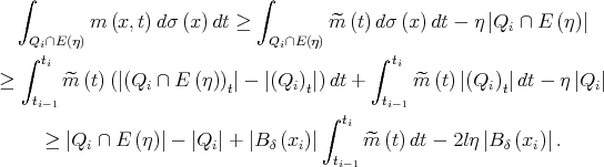
 and
and  we get
  ). So, the above inequalities give

 Thus
Thus 

For  let
let  From (68) and (69) we have
Hence 
where  and
and  denote the cardinals of
  and
and  respectively. Since
  and Lemma 3.11 gives that
  taking
  large enough and
  and
and  small enough the lemma follows.
For a  periodic curve
  and
and  let
let  defined by (64). We have
Lemma 5.3. Assume that  is connected. Then for each
  there exist
  and
and  such that
Proof. Let  and let
 and
and  be as in Lemma 5.2. For
  and
and  let
let ![γ : [t - θ,t + θ] → ∂ Ω i i i](/img/revistas/ruma/v46n2/2a051517x.png) be a
be a  map satisfying
 and
and  for
for  and
and  Let
Let  be defined by
  for
for ![t ∈ [t0,t1 - θ],](/img/revistas/ruma/v46n2/2a051526x.png)
 for
for ![t ∈ [tn + θ,tn]](/img/revistas/ruma/v46n2/2a051528x.png) and by
and by
for  For
For  small enough
  satisfies the conditions of the lemma.
Corollary 5.4. Assume that  is connected and let
  be defined by (6). If
  then for
  positive and small enough there exists
  such that
Remark 5.5. Let  as in Lemma 5.3. Since the map
  belongs to
  there exists a
  and
and  periodic map
  from
from  into
into  such that
  for
for  . Let
. Let  be an orthonormal basis of
  and let
  for
for 
 . Thus each
  is a
is a  periodic map,
  and for each
 is an orthonormal basis of
  For
For  and
and  we set
and 
(70) 
(71)
For  let
let  and
and  . Thus, for
  positive and small enough
  is a diffeomorphism from
  onto an open neighborhood
  of the set
  satisfying


 is
is  periodic in
Moreover,  and its inverse
  are of class
  on their respective domains. For
  as above, with
 we have
  and also (cf. (3.13) and (3.14) in [8])

for some  satisfying
  for
for  and
and  for
for  . Moreover, if
  denotes the Jacobian matrix of
  at
at  from the definition of
  and taking into account that the differential of
  at the origin is the identity on
  we have that
  for
for  .
.
Lemma 5.6. Assume that  is connected and that
  Then
Then 
Proof. Let  be a sequence in
  that converges to
  a.e in
  and satisfying
  for
for  let
let  be a sequence of operators as in Lemma 2.8 and let
  be the
  matrix whose
  entry
entry  , let
, let  be a sequence in
  for some
  and such
 in
in  .
.
For  positive and small enough let
  be as in Corollary 5.4 and let

 and
and  be as in Remark 5.5.
For  let
let
let  with
with
and let  be the
  symmetric and positive matrix whose
  entry is
  let
let  be defined on
  by
by  let
let 
 be defined on
 ![D δ × {0} × [0,T]](/img/revistas/ruma/v46n2/2a051641x.png) by
by  and
and  For
For  let
let  be a positive and
  periodic solution of
normalized by  Let
Let  be defined by
  Then, a computation shows that
Let  (to be chosen latter), let
  such that
 for
for 
 for
for  and let
  be defined by
  for
for  Finally, we set
  and, for a definite positive matrix
  and
and  we put
  With these notations we have, as in the proof of Lemma 3.11 in [8],
Also ![∫ ( 2 ) μmn,L(n),b(n0)(λ) G ^g (ξ, 0,t) dξdt D δ×(0,T) ∫ ( ) ≤ - λ G2 ^gm^n (ξ,0,t)dξdt [ Dδ×(0,T) ] ∫ ∥∥ ( G ) ∥∥2 + ∥∥ ∇G + --A^(n)^b(n) ∥∥ + ^a(n0)(s,t)G2 (s,t) dsdt. {s∈ℝN:∣s∣< δ:}×(0,T) 2 A^(n)(s,t)](/img/revistas/ruma/v46n2/2a051666x.png)
(72)
Thus, since  and
and  is continuous, we get
  for
for  positive and small enough. Then (for a smaller
  if necessary) and some positive constant
  we have
for  large enough. Since
  is continuous on
  and
and  we can assume also (diminishing
  and
and  if necessary) that, for
  large enough,

¿From these inequalities it is clear that we can pick  small enough in the definition of
  such that for
  large enough
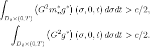
(73)
(74)
We have also
so, from (73), we get positive constants  and
and  independent of
  and
and  such that
  for all
  large enough. Also, since
Lemma 4.3 gives  Thus
Thus  is bounded, and so, after pass to a subsequence we can assume that
  converges to some
  . Since
  is bounded in
  by Lemma 3.3 and after pass to a furthermore subsequence, we can assume that
  converges in
  to some
  By Lemma 2.8
  satisfies
  in
in  ,
,  on
on  Thus
Thus  and so
  .
.
6. Principal eigenvalues for periodic parabolic Steklov problems
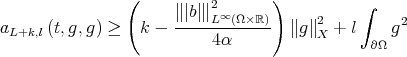
Let  and
and  be defined by (6). We have
Theorem 6.1. Suppose one of the following assertions i), ii), iii), holds.
i)  (respectively
  ) and either
  or
or 
ii) 
 (respectively
  ),
),  (resp.
  ) with
  defined as in remark 3.7.
Then there exists a unique positive (resp. negative) principal eigenvalue for (55) and the associated eigenspace is one dimensional.
Proof. Suppose 

 and
and  Since
Since  and, by Lemma 3.14,
  the existence of a positive principal eigenvalue
  for (55) follows from Lemma 5.6. Since
  does not vanish identically, the concavity of
  gives the uniqueness of the positive principal eigenvalue.
Moreover, if  are solutions in
  for (55), then, from Lemma 4.1,
  on
on  for some constant
  Since, for
  ,
,  on
on 
 and
and  on
on  . Thus, taking
  large enough, Lemma 2.9 gives
  on
on 
If either  or
or  then (by Remark 3.12)
  and so the existence follows from Lemma 5.6. The other assertions of the theorem follow as in the case
  Since
Since  and
and  the assertions concerning negative principal eigenvalues reduce to the above.
Theorem 6.2. Let  such that
  Then for all
  the problem
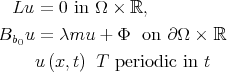
(75)
has a unique solution. Moreover  implies that
Proof. Since  for
for  large enough we have
  and so ,
  is a well defined and positive operator. If
  is a solution of (75) then
  so the solution, if exists, is unique. To see that it exists, consider
and observe that  solves (75). Finally, if
  then
then  on
on  and since

Lemma 2.18 (iii) gives 
Let  (respectively
  ) be the positive (resp. negative) principal eigenvalue for the weight
  with the convention that
  (respectively
  ) if there not exists such a principal eigenvalue. From the properties of
  Theorem 6.2 gives the following
Corollary 6.3. Assume that either  or
or  Then the interval
  does not contains eigenvalues for problem (55). If
  and
and  the same is true for the intervals
  and
and 
[1] Amann, H., Fixed point equations and nonlinear eigenvalue problems in ordered Banach spaces, SIAM Review, Vol. 18, No 4, (1976), 620-709. [ Links ]
[2] Beltramo, A. and Hess, P. On the principal eigenvalues of a periodic -parabolic operator , Comm. in Partial Differential Equations 9, (1984), 914-941. [ Links ]
[3] Crandall, M.G. and Rabinowitz, P. H., Bifurcation, perturbation of simple eigenvalues and stability, Arch. Rat. Mech. Anal. V. 52, No2, (1973) 161-180. [ Links ]
[4] Hess, P., Periodic Parabolic Boundary Problems and Positivity, Pitman Research Notes in Mathematics Series 247, Harlow, Essex, 1991. [ Links ]
[5] D. Daners and P. Koch-Medina, Abstract evolution equations, periodic problems and applications, Pitman Research Notes in Mathematics Series 279. Harlow, Longman Scientific & Technical, New York Wiley (1992). [ Links ]
[6] Hungerbulher, N., 'Quasilinear parabolic system in divergence form with weak monotonicity, Duke Math. J. 107/3 (2001), 497-520. [ Links ]
[7] T. Godoy, E. Lami Dozo and S. Paczka, The periodic parabolic eigenvalue problem with  weight, Math. Scand. 81 (1997), 20-34. [ Links ]
[8] T. Godoy, E. Lami Dozo and S. Paczka, Periodic Parabolic Steklov Eigenvalue Problems, Abstract and Applied Analysis, Vol 7, N 8, (2002) 401-422. [ Links ]
[9] Ladyžsenkaja, O. A. - Solonnikov and V. A., Ural'ceva, N. N., Linear and quasilinear equations of parabolic type, Translations of Mathematical Monographs, Vol. 23, American Mathematical Society, Providence, Rhode Island (1968).
[10] Lions, J. L. Quelques méthodes de résolution des problemès aux limites non linéaires, Dunod, Paris (1964). [ Links ]
[11] Miguel de Guzmán, Differentiation of integrals in  , Lectures Notes in Math. 481, Springer, Berlin (1975). [ Links ]
[12] Tanabe, H., Equations of evolution,Translated from Japanese by N. Mugibayashi and H. Haneda, (English), Monographs and Studies in Mathematics 6. London - San Francisco - Melbourne: Pitman. XII, (1979). [ Links ]
[13] M. Zerner, Quelques propriétés spectrales des opérateurs positifs, J. Funct. Anal. 72 (1987), 381-417. [ Links ]
T. Godoy
Facultad de Matemática, Astronomía y Física and CIEM - Conicet,
Universidad Nacional de Córdoba,
Ciudad Universitaria,
5000 Córdoba, Argentina
godoy@mate.uncor.edu
E. Lami Dozo
Département de Mathématique,
Université Libre de Bruxelles and
Universidad de Buenos Aires - Conicet,
Campus Plaine 214, 1050 Bruxelles
lamidozo@ulb.ac.be
S. Paczka
Facultad de Matemática, Astronomía y Física and CIEM - Conicet,
Universidad Nacional de Córdoba,
Ciudad Universitaria,
5000 Córdoba, Argentina
paczka@mate.uncor.edu
Recibido: 16 de diciembre de 2005
Aceptado: 7 de agosto de 2006

