


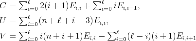
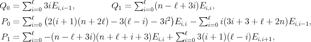
Serviços Personalizados
Journal

Artigo
 Inglês (pdf)
 Artigo em XML
 Referências do artigo
 Enviar este artigo por email
Indicadores
-
 Citado por SciELO
Links relacionados
-
 Similares em
SciELO
Similares em
SciELO
Compartilhar

 Permalink
Revista de la Unión Matemática Argentina
versão impressa ISSN 0041-6932versão On-line ISSN 1669-9637
Rev. Unión Mat. Argent. v.49 n.2 Bahía Blanca jul./dez. 2008
Matrix spherical functions and orthogonal polynomials: An instructive example
I. Pacharoni
This paper is partially supported by CONICET, FONCyT, Secyt-UNC and the ICTP.
Abstract. In the scalar case, it is well known that the zonal spherical functions of any compact Riemannian symmetric space of rank one can be expressed in terms of the Jacobi polynomials. The main purpose of this paper is to revisit the matrix valued spherical functions associated to the complex projective plane to exhibit the interplay among these functions, the matrix hypergeometric functions and the matrix orthogonal polynomials. We also obtain very explicit expressions for the entries of the spherical functions in the case of 2 × 2 matrices and exhibit a natural sequence of matrix orthogonal polynomials, beyond the group parameters.
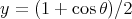
The well known Legendre polynomials are a special case of spherical harmonics: the homogeneous harmonic polynomials of  , considered as functions on the unit sphere
  . Let
. Let  be ordinary polar coordinates in
  :
: 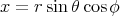 ,
, 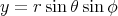 and
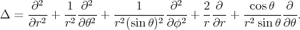
and  In terms of these coordinates the Riemannian structure of
  is given by the symmetric differential form
  and the Laplace operator is
 is a homogeneous harmonic polynomial of degree
  which does not depend on the variable
  , then
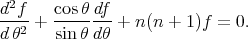
 we get
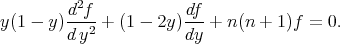
 , up to a constant, is
 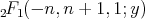 . Since the Legendre polynomial of degree
  is given by
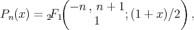
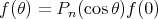 .
. Let
 be the north pole of
  , and let
  be the geodesic distance from a point
  to
to  . Let
. Let 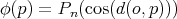 . Then we have proved that
  is the unique spherical harmonic of degree
  , constant along parallels and such that
  . Moreover the set of all complex linear combinations of translates
 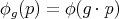 ,
,  , is the linear space of all spherical harmonics of degree
  .
. Legendre and Laplace found that the Legendre polynomials satisfy the following addition formula
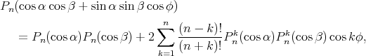 (1) (1) |
where the  's are the associated Legendre polynomials.
By integrating (1) we get
 (2) (2) |
Moreover the Legendre polynomials can be determined as solutions to (2). This integral equation can now be expressed in terms of the function  on
on  defined by
  . In fact (2) is equivalent to
 (3) (3) |
where  denotes the compact subgroup of
  of all elements which fix the north pole
  , and
, and  denotes the normalized Haar measure of
  .
.
In fact, let  denote the subgroup of all elements of
  which fix the point
  . Then
 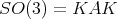 . Thus to prove (3) it is enough to consider rotations
  and
and  around the
  -axis through the angles
  and
and  , respectively. Then if
  denotes the rotation of angle
  around the
  -axis we have

 and
and 
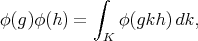
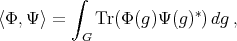
The functional equation (3) has been generalized to many different settings. One is the following. Let  be a locally compact unimodular group and let
  be a compact subgroup. A nontrivial complex valued continuous function
  on
on  is a zonal spherical function if (3) holds for all
  . Note that then
 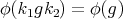 for all
  and all
  , and that
  where
where  is the identity element of
  .
.
The example above arises when 
 and
and  . The other compact connected rank one symmetric spaces have zonal spherical functions which are orthogonal polynomials in an appropriate variable. These polynomials are special cases of Jacobi polynomials and they can be given explicitly as hypergeometric functions.
The complex projective plane 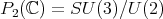 is another rank one symmetric space. In this case the zonal spherical functions are
  .
.
A very fruitful generalization of the functional equation (3) is the following (see [T1] and [GV]. Let  be a locally compact unimodular group and let
  be a compact subgroup of
  . Let
. Let  denote the set of all equivalence classes of complex finite dimensional irreducible representations of
  ; for each
  , let
, let  and
and  denote, respectively, the character and the dimension of any representation in the class
  , and set
  . We shall denote by
  a finite dimensional complex vector space and by
  the space of all linear transformations of
  into
into  .
.
A spherical function  on
on  of type
  is a continuous function
  such that
  , (
, ( = identity transformation) and
When  is the class of the trivial representation of
  and
and  , the corresponding spherical functions are precisely the zonal spherical functions. From the definition it follows that
  is a representation of
  , equivalent to the direct sum of
  representations in the class
  , and that
  for all
  and all
  . The number
  is the height of
  . The height and the type are uniquely determined by the spherical function.
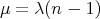
2. Matrix valued spherical functions associated to 
In [GPT1] the authors consider the problem of determining all irreducible spherical functions associated to the complex projective plane  . This space can be realized as the homogeneous space
  ,
,  and
and  . In this case all irreducible spherical functions are of height one. Let
  be any irreducible representation of
  in the class
  . Then an irreducible spherical function can be characterized as a function
  such that
 is analytic,
 , for all
  ,
,  , and
, and  ,
, = λ(Δ )Φ (g )](/img/revistas/ruma/v49n2/2a02124x.png) , for all
, for all  and
and  .
.
Here  denotes the algebra of all left and right invariant differential operators on
  . In our case it is known that the algebra
  is a polynomial algebra in two algebraically independent generators
  and
and  , explicitly given in [GPT1].
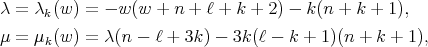
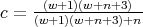
The set  can be identified with
  in the following way: If
  then
then

 denotes the
  -symmetric power of the matrix
  .
. For any  we denote by
  the left upper
  block of
  , and we consider the open dense subset
  . Then
  is left and right invariant under
  . For any
  we introduce the following function defined on
  :
:
 above denotes the unique holomorphic representation of
  which extends the given representation of
  .
. To determine all irreducible spherical functions  of type
  , we use the function
  in the following way: in the open set
  we define the function
  by
by
 (4) (4) |
where  is supposed to be a spherical function of type
  . Then
  satisfies
 ,
, , for all
  ,
, , for all
  .
.
The canonical projection  defined by
  where
where  maps the open dense subset
  onto the affine space
  of those points in
  whose last homogeneous coordinate is not zero. Then property ii) says that
  may be considered as a function on
  , and moreover from iii) it follows that
  is determined by its restriction
  to the cross section
  of the
  -orbits in
  , which are the spheres of radius
  centered at the origin. That is
  is determined by the function
  on the interval
  . Let
. Let  be the closed subgroup of
  of all diagonal matrices of the form
  ,
,  . Then
  fixes all points
  . Therefore iii) also implies that
  for all
  . Since any
  as an
as an  -module is multiplicity free, it follows that there exists a basis of
  such that
  is simultaneously represented by a diagonal matrix for all
  . Thus, if
  , we can identify
  with a vector

 is an eigenfunction of
  and
and  makes
makes  into an eigenfunction of certain differential operators
  and
and  on
on  .
. Making the change of variables  these operators become
If we denote by  the
the  matrix with entry
  equal to 1 and 0 elsewhere, then the coefficient matrices are
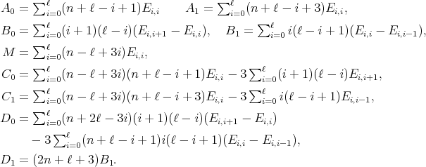
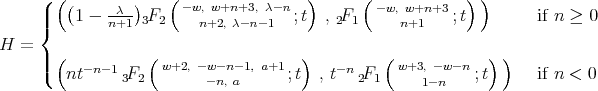
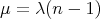
The following result, which characterizes the spherical functions associated to the complex projective plane is taken from Theorem 3.8 of [RT], see also [GPT1].
Theorem 2.1. The irreducible spherical functions  of
of  of type
  , correspond precisely to the simultaneous
  -valued polynomial eigenfunctions
  of the differential operators
  and
and  , introduced in (5) and (6), such that
  for all
  with
with  polynomial and
  .
.
We also obtain, from [GPT1] or [PT1], that there is a bijective correspondence between the equivalence classes of all irreducible spherical functions  of type
  and the set of pairs of integers
 (7) (7) |
Under this correspondence the function  associated to the spherical function
  satisfies
  and
and  where
where
 (8) (8) |
2.1. Hypergeometric operators. A key result to characterize the spherical functions of  of any type
  is the fact that the differential operator
  is conjugated, by a matrix polynomial function
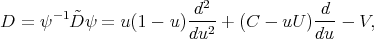
  , to a hypergeometric operator
  . From [RT], (or [PT2], for a more general situation) we obtain that the function
  , where
 takes the hypergeometric form
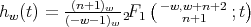
  (9) (9) |
where the coefficient matrices are 
This fact allows us to describe the eigenfunctions of the differential operator  in term of the matrix valued hypergeometric functions, introduced in [T2]: Let
  be a
be a  -dimensional complex vector space, and let
  and
and  . The hypergeometric equation is
where  stands for a function of
  with values in
  .
.
More generally we can consider the equation
 (11) (11) |
In the scalar case the differential operator (11) is always of the form (10). Nevertheless in a noncommutative setting the equations  and
and  may have no solutions
  ,
,  .
.
If the eigenvalues of  are not in
  we define the function
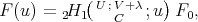
![( ) ∞∑ m 2H1 U ;V;z = z--[C; U ;V]m, C m=0 m!](/img/revistas/ruma/v49n2/2a02257x.png) (12) (12) |
where the symbol ![[C,U, V ]m](/img/revistas/ruma/v49n2/2a02258x.png) is defined inductively by
is defined inductively by ![[C; U ;V ]0 = I](/img/revistas/ruma/v49n2/2a02259x.png) and
and
![[C; U ;V] = (C + m )-1(m2 + m (U - 1) + V)[C; U;V ] , m+1 m](/img/revistas/ruma/v49n2/2a02260x.png) |
for all  . The function
  is analytic on
  , with values in
  . Moreover if
  then
then 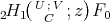 is a solution of the hypergeometric equation (11) such that
  . Conversely any solution
  of (11), analytic at
  is of this form.
2.2. Spherical functions as matrix hypergeometric functions. The irreducible spherical functions of  of type
  are in a one to one correspondence with certain simultaneous
  -polynomial eigenfunctions
  of the differential operators
  and
and  (see Theorem 2.1).
A delicate fact establish in [RT] is that the functions  are also polynomials functions which are eigenfunctions of the differential operators
  and
and  .
.
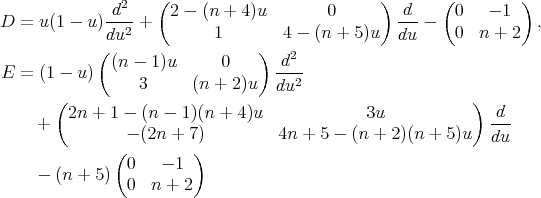
In the variable  , these operators have the form
 (13) (13) |
 (14) (14) |
where the coefficient matrices are
 | (15) |
To describe all simultaneous  -polynomial eigenfunctions of the differential operators
  and
and  we start by considering the eigenfunctions of
  of eigenvalues
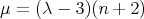
  , with
  (see (8)). We let

Remark. It is not difficult to prove that that  if and only if
  , for some
  .
.
Therefore if  then it is of the form
 . The simultaneous eigenfunctions of
  and
and  will correspond to particular choices of
  .
. Since the initial value  determines
  , we have that the linear map
 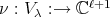 defined by
  is a surjective isomorphism. Since
  and
and  commute, the differential operators
  and
and  also commute. Moreover, since
  has polynomial coefficients whose degrees are less or equal to the corresponding orders of differentiation,
  restricts to a linear operator of
  . Thus we have the following commutative diagram
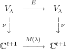 (16) (16) |
where  is the
  matrix given by
 (17) (17) |
The eigenvalues of  are given by (see Theorem 10.3 in [GPT1])

 of
of  have geometric multiplicity one. In other words all eigenspaces are one dimensional. Moreover if
 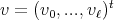 is a nonzero
  -eigenvector of
  , then
  .
. The irreducible spherical functions of  of type
  are parameterized by two nonnegative integers
  with
with  and
and 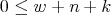 (see (7)). Under this correspondence the function
  associated to the spherical function satisfies
  and
and  where
where
 (18) (18) |
Then the characterization of the irreducible spherical functions is summarize in the following theorem, taking from [RT].
Theorem 2.2. The function  associated to a spherical function of type
  and parameters
  is of the form
 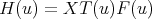 , where
 (19) (19) |
and  is the unique
  -eigenvector of
  normalized by
  . The expressions of the matrices
  are given in (15) and the eigenvalues
  and
and  are given in (18).
2.3. Orthogonality. Let  be the space of all continuous functions
  such that
  for all
  ,
,  . Let us equip
  with an inner product such that
  becomes unitary for all
  . We have the following inner product in
  :
:
 (20) (20) |
where  denotes the adjoint of
  with respect to the inner product in
  . Then we have the following inner product on the corresponding functions
  's associated to the spherical functions
 (21) (21) |
where
Since the Casimir operator is symmetric with respect to the  -inner product for matrix valued functions on
  given in (20), it follows that the differential operators
  and
and  are symmetric with respect to the weight function
  , that is they satisfy
Now it is easy to verify that the differential operators  and
and  are symmetric with respect to the weight function
 (22) (22) |
To illustrate the above result we will display the cases  (the scalar case) and
  , where the size of our matrices will be
  .
.
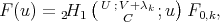
3.1. The case  .. In this case the functions
  are scalar functions. If the parameter
  is 0 then we have the zonal spherical functions.
The operator  is proportional to
  , (
, ( ) and
) and

 we put
 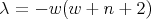 . Then
  should be a solution of the hypergeometric equation with
 |
are linearly independent solutions. By Theorem 2.1 we have that  should be a polynomial function such that
  . Moreover if
  the function
  have to satisfies
 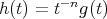 with
with  a polynomial function. Therefore we get: For
  and
and 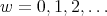
 and
and 

 , for
, for  and
and  .
. By using the Pfaff's identity we get


Therefore we obtain that
Proposition 3.1. The spherical functions associated to the complex projective plane of type  are
are

 ,
,  and
and  . Moreover these functions satisfy
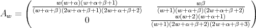
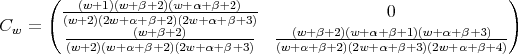
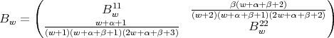
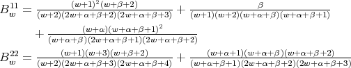
3.2. The case  . In this case the operators
  and
and  are
are 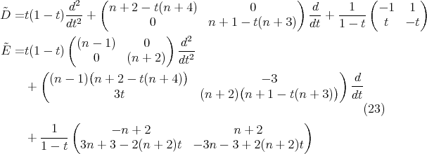
In [GPT1], Section 11.1 we exhibit the complete list of spherical function of type  . We have two families of such functions, corresponding with the choice of the parameter
  or
or  . For
. For  the parameter
  is in the range
  , and if
 .
.
First family. For  we have
 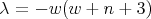 ,
,  . The (vector valued) function
  is given by, up to the normalizing constant such that
 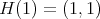 .
.
with  .
.
Second family. For  we have
  and
and  . The functions
  is
is
with  .
.
By taking the Taylor expansion at  these functions takes the following unified expression. We recall that
  corresponds to the identity of the group
  .
.
Theorem 3.2. The complete list of spherical functions associated to  of type
  are given by
- For
 we have
 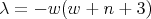 ,
,  and
and 
The parameter
 is an integer that satisfies
  and
and  .
. - For
 , we have
  ,
,  and
and 
where
 .
.
The parameter is an integer that satisfies
  and
and  .
.
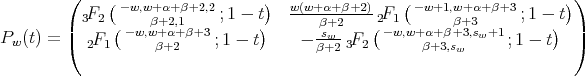
In this case the function  , where
  and
and  is
is
 (24) (24) |
In the variable  , the conjugated operators
  and
and  are
are
 (25) (25) |
The matrix  (see (17)), is
 are
are  and
and  and the respective normalized eigenvectors are
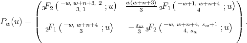
 associated to the spherical functions are, for
  ,
, 
 ,
, 
The explicit expression of the entries of these functions  's are given in the following theorem.
Theorem 3.3. The functions  associated to the spherical functions of the pair
 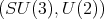 of type
  are given by
- For
 we have
  ,
,  and
and 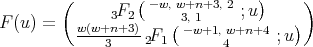
The parameter
 is an integer that satisfies
  and
and  .
. - For
 , we have
  ,
,  and
and where
 .
.
The parameter is an integer that satisfies
  and
and  .
.
Proof. If  is an eigenfunction of
  then
then  is an eigenfunction of
  with the same eigenvalue. Explicitly the function
  is
is
 (26) (26) |
From
 |
(26) we only have to prove the expression for the second entry of the function  . For the first family, from Theorem 3.2 we get
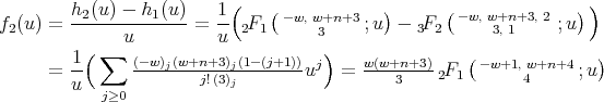
For the second family we obtain, with 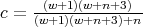
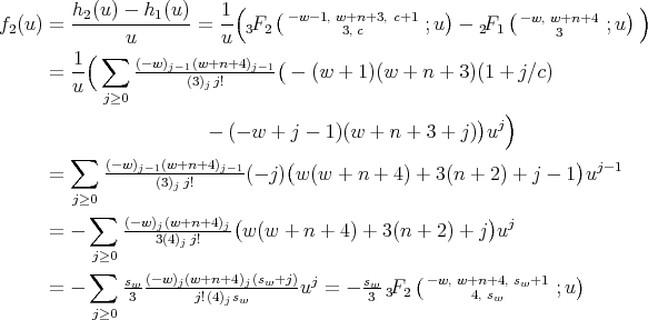
This concludes the proof of the theorem. □
3.3. Matrix valued orthogonal polynomials coming from spherical functions. In the scalar case, it is well known that the zonal spherical functions of the sphere 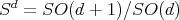 are given, in spherical coordinates, in terms of Gegenbauer polynomials. Therefore, it is not surprising that in the matrix valued setting the same phenomenon occurs: the matrix spherical functions are closely related to matrix orthogonal polynomials.
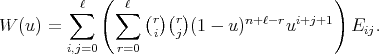
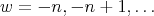
For a given nonnegative integers  and
and  we define the matrix polynomial
  as the
  matrix function whose
  -row is the polynomial
  , associated to the spherical functions of type
  , given in the previous section. In other words
 .
. Since different spherical functions are orthogonal with respect to the natural inner product among these functions, we obtain that the matrices  are orthogonal with respect to the weight function
  :
:
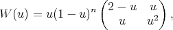

 is a triangular nonsingular matrix. Therefore
  is a sequence of matrix valued orthogonal polynomials with respect to the weight matrix
  .
. The columns of  are eigenfunctions of the differential operators
  and
and  given in (25), thus we have that
  satisfies

 and
and  are
are 
3.4. Extension of the group parameters. These results have a direct and fruitful generalization by replacing the complex projective plane by the  -dimensional complex projective space
  , which can be realized as the homogeneous space
  , where
  and
and  .
.
In this case, the finite dimensional irreducible representations of  , are parameterized by the
  -tuples of integers
  such that
  . By considering the irreducible spherical functions of type
 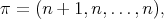 and proceeding as we explained for the complex projective plane, one obtains a situation that generalizes the one of
  . Then by extending the parameters
  ,
,  we have the following results.
Theorem 3.4. Let 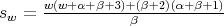 and let us define
Then
 is a sequence of orthogonal polynomials with respect the weight matrix
Let  be the following second order differential operator

 satisfies
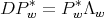

In [PT1] for  or in general in [P08], we obtain a multiplication formula for spherical functions by tensoring certain irreducible representations of
  and decomposing them into irreducible representations. From this formula we derive a three term recursion relation for the "packages" of spherical functions. Restricting this to the variable
  (the variable that parameterizes a section of the
  -orbits in
  ), we obtain a three term recursion relation for the packages of functions
  associated to the spherical functions. In this case we obtain the following
Theorem 3.5. The sequence  satisfies the following three term recursion relation
 |
with
Remark 3.6. The three term recursion relation can be seen as a difference operator in the variable  , given by a semiinfinite matrix
  . The vector matrix
  is an eigenfunction of
  because it satisfies
  .
.
We observe that the semiinfinte matrix  have the interesting property that the sum of all the matrix elements in any row is equal to one. Moreover all the entries of
  are nonnegative real numbers. This have important applications in the modeling of some stochastic phenomena.
[GV] Gangolli R. and Varadarajan V. S. Harmonic analysis of spherical functions on real reductive groups, Springer-Verlag, Berlin, New York, 1988. Series title: Ergebnisse der Mathematik und ihrer Grenzgebiete, 101. [ Links ]
[GPT1] F. A. Grünbaum, I. Pacharoni and J. Tirao, Matrix valued spherical functions associated to the complex projective plane, J. Funct. Anal. 188 (2002), 350-441. [ Links ]
[P08] Pacharoni I.Three term recursion relation for spherical functions. Preprint, 2008. [ Links ]
[PT1] Pacharoni I. and Tirao J. A. Three term recursion relation for spherical functions associated to the complex projective plane. Math Phys. Anal. Geom. 7 (2004), 193-221. [ Links ]
[PT2] Pacharoni I. and Tirao J. A. Matrix valued orthogonal polynomials arising from the complex projective space. Constr. Approxim. 25, No. 2 (2007) 177-192. [ Links ]
[PR] Pacharoni, I. Román, P. A sequence of matrix valued orthogonal polynomials associated to spherical functions Constr. Approxim. 28, No. 2 (2008) 127-147. [ Links ]
[RT] P. Román and J. A. Tirao. Spherical functions, the complex hyperbolic plane and the hypergeometric operator. Intern. J. Math. 17, No. 10, (2006), 1151-1173. [ Links ]
[T1] J. Tirao. Spherical Functions. Rev. de la Unión Matem. Argentina, 28 (1977), 75-98. [ Links ]
[T2] J. Tirao, The matrix-valued hypergeometric equation. Proc. Natl. Acad. Sci. U.S.A., 100 No. 14 (2003), 8138-8141. [ Links ]
I. Pacharoni
CIEM-FaMAF,
Universidad Nacional de Córdoba,
Córdoba 5000, Argentina
pacharon@mate.uncor.edu
Recibido: 18 de mayo de 2008
Aceptado: 11 de agosto de 2008

