


 Inglês (pdf)
 Artigo em XML
 Referências do artigo
 Enviar este artigo por email
 Citado por SciELO
  Similares em
SciELO
Similares em
SciELO 
 Permalink
Introduction
The hydraulic conductivity represents the ability of a porous medium to transmit water through its interconnected voids (Alyamani and §en, 1993). Hydrologists have been concerned with the determination of relationships between hydraulic conductivity and grain-size distribution parameters since the work by Hazen (1893). The analysis of grain-size distribution (sorting) has been in turn of interest to geologists since its introduction by Krumbein and Monk (1943), because the grain-size is the most fundamental property of sediment particles affecting their entrainment, transport and deposition (Blott and Pye, 2001). Up to the present, a variety of different empirical approaches are available to estimate the permeability (i.e., hydraulic conductivity) of a sediment from its grain-size distribution (Rosas et al, 2013). Alternatively, the permeability can be determined in the laboratory using permeameters as well as by classical analytical methods involving in situ pump tests. However, accurate estimation of the permeability in the field environments is limited by the lack of precise knowledge of aquifer geometry and hydraulic boundaries (Uma et al, 1989; Unnikrishnan et al, 2016). Laboratory tests, on the other hand, can be problematic in the sense of obtaining representative samples and they need, very often, long testing times (Odong, 2007). In hydromechanics, it would be more useful to characterize the diameters of pores rather than those of the grains, but the pore size distribution is very difficult to determine and thus the approximation of hydraulic properties is mostly based on the easy-to-mea-sure grain-size distribution as a substitute (Cir-pka, 2004). And also, in other fields of research such as chemistry and engineering, grain-size distribution, particle shape (Tickell and Hiatt, 1938), and particle packing (Tickell and Hiatt, 1938; Furnas, 1931) have been indicated to explain variations in porosity and permeability.
It has become increasingly important to being able to accurately estimate the hydraulic conductivity of unlithified sediments for different engineer applications, such as natural filtration projects (Rosas et al, 2013) or the use of soil columns to assess the removal of pathogens, algae, and trace organic contaminants (Lewis and Sjostrom, 2010). At the same time, Alyamani and §en (1993) define the hydraulic conductivity as one of the most important characteristics of water-bearing formation since its magnitude, pattern and variability significantly influence the ground-water flow patterns and contaminants dissolved in the water through the soils (Salarashayeri and Siosemarde, 2012). Furthermore, streambed hydraulic conductivity is a primary factor controlling the efficiency of collector wells (Zhang et al, 2011), and is an important parameter in modelling the surface and ground water mixing in the hyporheic zones (Lautz and Siegel, 2006).
The objectives of this study were to (1) apply 11 empirical formulas to calculate hydraulic conductivity of unconsolidated river sediments from grain-size distribution, and (2) compare and select a suitable empirical formula among them for further estimating the hydraulic conductivity of hyporheic sediments. For this purpose, we measured sediment grain-size distribution from 36 sandy sediment samples, collected from a fluvial channel, and estimated sediment physical characteristics such as the texture, the effective diameter, the coefficient of uniformity and the defined porosity. Based on these sediment physical characteristics, we calculated hydraulic conductivity by applying those different empirical formulas. In addition, we reviewed the limits of the applicability for each formula.
Material and Methods
Collection of sediment samples
The fieldwork of this study was conducted at the downstream reach (about kilometre 54 from the source) of the Tordera River (a 3rd order Mediterranean river located at the north-east of the Iberian Peninsula). Three sampling campaigns were performed (December 2012, June and July 2013). On each sampling campaign, sandy sediment samples from four different sites were collected by using a Multisampler (reference 12.41, Eijkelkamp, Giesbeek, The Netherlands) to obtain sediment core samples from surface to 60 cm depth. For each site, the sediment was divided into three fractions (0-5, 20-30, and 50-60 cm depths). The sediment was dried (105°C, 24 h) and grain-size distribution was analysed.
Sedimentgrain-size measurements
The grain-size analysis of the collected sediment samples was performed following the American Society for Testing and Materials [i.e., the sieving and hydrometer tests of the ASTM method D422-63 (reapproved 1998)]. This method covers the quantitative determination of the distribution of grain sizes in soils. In our sediment samples, there were very few grain sizes greater than 9.5 mm in diameter found at each depth of all sites. A representative sample of the sediments (about 300 g of dry weight) was run through a set of ASTM E11 sieves (9.5, 4.75, 3.35, 2,1.18, 0.6, 0.3, 0.15, and 0.075 mm) to break the sample subset into size classes by dry sieving for the coarser fractions, when the finer size fractions (< 0.075 mm diameter) were determined by sedimentation process using an ASTM 152-H hydrometer. In this latter case, the sample (about 100 g of dry weight < 2 mm diameter) was placed in a beaker of 250 mL volume and covered with 125 mL of sodium hexametaphosphate solution [40 g (NaPO3)6/L distilled water]. After soaking, at least 16 hours, the soil-water slurry was dispersed for a period of 1 min with a magnetic stirrer. Immediately after dispersion, all the soil-water slurry was transferred in the glass sedimentary cylinder. The cylinder was refilled with distilled water until the total volume of 1000 mL. The soil-water slurry was well mixed by turning the cylinder upside down approximately 60 turns for a period of 1 min to complete the agitation of the slurry. After mixing, the slurry cylinder was placed in a constant-temperature compartment where a 1000 mL blank cylinder (i.e., to measure the zero correction which can be positive or negative) had been prepared with 125 mL of sodium hexametaphosphate solution and 875 mL of distilled water. Then, the readings were performed (about 20 to 25 s after each time we inserted the hydrometer to be freely floating without touching the wall of the sedimentation cylinder) at 2, 5, 15, 30, 60, 250, and 1440 min as well as the temperature of the suspension with an accurate to 0.5 oC thermometer registered. From the hydrometer readings, the diameter of particles was estimated by the Stoke’s law [sensus Murthy (2002)].
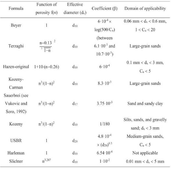
Table 1: Grain-size empirical formulasa and their applicability domain for the determination of the hydraulic conductivity (K) in cm/s. The general empirical formula takes the form of K = (g/n).β.f(n).dx2 in which: n - kinematic viscosity is set to 1.002·10-2 cm2/s at 20oC when g - the acceleration due to gravity is equal to 980 cm/s2. dx (cm) - the value (originally read in mm) is defined as the effective diameter with x % cumulative weight of the sample which is determined by the grain-size distribution curve (Lu et al., 2012). n is porosity derived from the empirical formula with the coefficient of uniformity (Vukovic and Soro, 1992): n = 0.255 . (1+0.83Cu) where Cu is the coefficient of uniformity and is defined as Cu = d60/d10 (Holtz and Kovacs, 1981). d60 and d10 represent the grain diameter (mm) for which, 60 % and 10 % of the sample respectively, are finer than, which are readily obtained from the grain-size distribution curve (Abdullahi, 2013). USBR stands for the U.S Bureau of Reclamation. / Tabla 1: Formula empírica de la granulometría y su aplicación para la determinación de la conductividad hidráulica (K) en cm/s. La fórmula empírica general toma la forma de K = (g/n).β.f(n).dx2 donde: n - la viscosidad cinemática se fija en 1.002·10-2 cm2/s a 20oC cuando g la aceleración debida a la gravedad es igual a 980 cm/s2. dx (cm) el valor (originalmente leído en mm) se define como el diámetro efectivo con x % de peso acumulado de la muestra que se determina por la curva de distribución del tamaño del grano (Lu et al., 2012). n es la porosidad derivada de la fórmula empírica con el coeficiente de uniformidad (Vukovic y Soro, 1992): n = 0,255 . (1+0,83Cu) donde Cu es el coeficiente de uniformidad y se define como Cu = d60/d10 (Holtz y Kovacs, 1981). d60 y d10 representan el diámetro del grano (mm) para el cual, el 60 % y el 10 % de la muestra, respectivamente, son más finos, lo que se obtienen fácilmente de la curva de distribución granulométrica (Abdullahi, 2013). USBR significa U.S. Bureau of Reclamation
For each sediment sample, several parameters were calculated from the grain-size distribution results with different empirical formulas (see Table 1, Eq. 1-2 and Eq. 3) by mediating the effective diameters and phi (0) sizes read at different percentages (Tables 2 and 3, respectively) - among others, geometric mean grain diameter (GM^), inclusive standard deviation (gJ, coefficient of uniformity (Cu), coefficient of curvature (Cc), defined porosity (n) and hydraulic conductivity (K).
Estimates of hydraulic conductivity
The hydraulic conductivity (K) of unconsolidated materials has been related empirically to grain-size distribution by a number of investigators (Hazen, 1893; Krumbein and Monk, 1943; Harleman, 1963; Masch and Denny, 1966; Wiebenga et a/., 1970), from which our study used a series of 11 empirical formulas to estimate the K values. Nine of them are described in Table 1 while other two are further defined as follows.
Krumbein and Monk (1943) proposed an empirical equation whose formula is nearly similar to the set of formulas given in Table 1. They used a statistical approach for the determination of the hydraulic conductivity (K) by using a transformation of the grain-size distribution to a logarithmic frequency distribution, and by incorporating various moments into an empirical equation (Rosas et a/., 2013). Their equation was empirically developed using very well sorted sediment samples ranging from -0.75 to 1.25 phi (0) in mean grain-sizes, and with standard deviations ranging from 0.04 to 0.80 phi (0). In this case, the calculation of the intrinsic permeability (k) from the grain-size analysis is determined experimentally as:
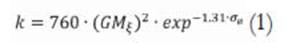
Where: k - intrinsic permeability in darcy, GM^ - geometric mean grain diameter (mm), o0 - the standard deviation of diameter in phi (0) scale. The geometric (graphic) mean is based on three points at specific percent coarser particles (by weight) and is equal to [(016+050+084)/3]. The inclusive (graphic) standard deviation, whose formula includes 90 % of the distribution that is calculated as [(084+016)/4 +(095+05)/6.6], is the best overall measure of sediment sorting. In order to facilitate graphical presentation and statistical manipulation of grain-size frequency data, Krumbein and Monk (1943) further proposed that grade scale boundaries should be logarithmically transformed into phi (0) values by using the expression phi (0) = -log2(d) where d is the grain diameter (mm). Distributions using these scales are termed “log-normal”, and are conventionally used by sedimentologists (Visher, 1969; Middleton, 1976).
The Krumbein and Monk’s permeability (k), in darcy, can be converted into the hydraulic conductivity (K), in cm/s, using the relation:
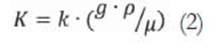
Where: k - intrinsic permeability, in units of cm2, is converted from Eq. 1 with the conversion factor (9.87.10-9 cm2/darcy); p - density of water (0.9982 g/cm3 at 20oC); g - acceleration of gravity (980 cm/s2); [j. - dynamic viscosity of water (0.01 g/cm.s at 20oC).
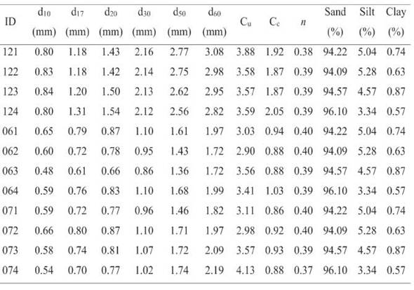
Table 2: Statistical parameters from the cumulative percent (passing) frequency distribution curves. These parameters were used to compute the hydraulic conductivity (K) as described in Table 1 and Eq. 3. Two prefix numbers in ID represent the sampling dates, e.g. 12 was December 2012, 06 was June 2013, and 07 was July 2013 while its suffixes represent the sampling sites. Values for each ID were calculated as an average from triplicate samples at surface (0-5 cm), 20 cm and 50 cm depths. dx (mm) value corresponds to which x % (e.g., read at 10, 17, 20, 30, 50, and 60 %) of the sample is finer, and was calculated from the phi (f) size formula given by Krumbein and Monk (1943). The coefficient of uniformity (Cu) for uniformly graded sediments containing grains of the same size is less than 4. Cc = d230/(d10.d60) called the coefficient of curvature lies between 1 and 3 for gravel and sands (Murthy, 2002). n is porosity of sediment expressed dimensionless in our calculation (see Table 1). / Tabla 2: Parámetros estadísticos de las curvas de distribución de frecuencias del porcentaje acumulado (de paso). Estos parámetros se utilizaron para calcular la conductividad hidráulica (K) como se describe en la Tabla 1 y la Ecuación 3. Dos números de prefijo en ID representan las fechas de muestreo, por ejemplo, 12 era diciembre de 2012, 06 era junio de 2013, y 07 era julio de 2013, mientras que sus sufijos representan los sitios de muestreo. Los valores para cada ID se calcularon como un promedio de muestras triplicadas en la superficie (0-5 cm), 20 cm y 50 cm de profundidad. El valor d (mm) corresponde a qué x % (por ejemplo, leído en 10, 17, 20, 30, 50 y 60 %) de la muestra es más fino, y se calculó a partir de la fórmula de tamaño phi (0) dada por Krumbein y Monk (1943). El coeficiente de uniformidad (C ) para los sedimentos uniformemente graduados que contienen granos del mismo tamaño es inferior a 4. Cc = d230/(d10.d60) llamado coeficiente de curvatura se encuentra entre 1 y 3 para las gravas y las arenas (Murthy, 2002). n es la porosidad del sedimento expresada sin dimensiones en nuestro cálculo (véase Tabla 1).
Another alternative procedure to estimate the hydraulic conductivity (K) from the grain-size analysis was that given by Alyamani and §en (1993). In this case, the proposed formula is clearly distinct to those listed in Table 1 and Eq. 2, and includes a variant from Hazen formulation (Hazen, 1893). The method relates the hydraulic conductivity, in cm/s, to the initial slope and intercept of the grain-size distribution curve, and is defined as:
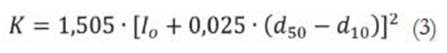
Where: I- the x-intercept (mm) of the straight line is formed by joining the mean grain diameter (d mm) and the effective diameter (d , mm) of the grain-size distribution curve, for which 50 % and 10 % of the grain sizes are
finer by weight, respectively.
Data analysis
The significant differences in hydraulic conductivity (K) from the different estimations were computed by a univariate analysis of variance followed by post-hoc comparisons using the Tukey’s HSD test differed at the P < 0.05 level. This was done independently for December, and June and July sampling dates. Furthermore, the Pearson’s r correlation coefficients between K obtained by different formulas were performed. The SPSS Statistics Vers.19 software was used for statistical analysis.
Results
The physical characteristics of the sediment samples collected in the Tordera River are summarized in Tables 2 and 3. Results showed that, after the hydrometer test, a small amount of mud (~ 4.6 % silt and 0.7 % clay) was recorded in our samples. Approximately 94.7 % of samples (by weight) were fallen in the coarser fraction (specifically, coarse sand, and very fine and fine gravel) for all sampling dates. Nearly all samples were uniformly graded due to their coefficient of uniformity (CJ less than 4, except a sample of site 4 in July (Cu ~ 4.13). On the other hand, the sand sediments had skewness values (Sk) in the range of 0.06 to 0.38 for December, -0.12 to 0.07 for June, and -0.14 to 0.11 for July while their kurtosis values (SG) ranged respectively from 1.32 to 1.94, 0.94 to 1.05, and 0.87 to 1.11 (all values not shown, their average is given in Table 3). In addition, the sorting of the grain sizes around the average was lying between the boundary of moderately and poorly sorted (Blott and Pye, 2001) for December (ct0 = 0.75-1.19), and for both June and July (ct0 = 0.96-1.31). Our sediment sample patterns in June and July coincided, and so their diameters at any percentage were approximately identical (see Figure 1D). Comparatively, coarser samples (> 0.075 mm diameter) in June and July showed smaller grain sizes than those in December (Tukey’s HSD test, P < 0.05, Figures 1 and 2).
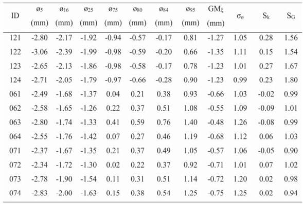
Table 3: Statistical parameters from the cumulative percent (retained) frequency distribution curves. See ID details’ description in Table 2. These parameters were used to compute the hydraulic conductivity (K) with the formula of Krumbein and Monk (see Eq. 2). The subscript in the phi terms (ox) refers the grain-size at which x % (e.g., read at 5, 16, 25, 75, 80, 84, and 95 %) of the sample is coarser than that size. As for the phi (0) size corresponding to the 50 % mark on the cumulative, either percent passing or retained, frequency distribution curves; the 05O values were estimated with the formula given by Krumbein and Monk (1943) (see the above-mentioned formula and use the d50 values in Table 2 for the calculation). Inclusive skewness (Sk) was used to describe the degree of asymmetry for a given distribution and is equal to [(016+084- 2.05O)/2 x (0 - 016)] + [(05+ 095-2.05O)/2 x (0 - 05)]. Graphic kurtosis (SG), used to describe the degree of peakedness for a given distribution, is defined as [(095- 05)/2.44 x (075- 025)] (Masch and Denny, 1966). / Tabla 3: Parámetros estadísticos de las curvas de distribución de frecuencias del porcentaje acumulado (retenido). Véase la descripción de los detalles de la identificación en el cuadro 2. Estos parámetros se utilizaron para calcular la conductividad hidráulica (K) con la fórmula de Krumbein y Monk (véase la ecuación 2). El subíndice en los términos phi (0J) se refiere al tamaño de grano en el que el x % (por ejemplo, leído en 5, 16, 25, 75, 80, 84 y 95 %) de la muestra es más grueso que ese tamaño. En cuanto a la talla phi (0) correspondiente a la marca del 50 % en las curvas de distribución de frecuencias acumulativas, ya sea de porcentaje de paso o de retención; los valores de 050 se estimaron con la fórmula dada por Krumbein y Monk (1943) (véase la fórmula mencionada y utilícese para el cálculo los valores d50 de la tabla 2). La asimetría inclusiva (Sk) se utilizó para describir el grado de asimetría de una distribución determinada y es igual a [(016+084- 2.050)/2 x (0^- 016)] + [(05+ 095-2.050)/2 x (095- 05)]. La curtosis gráfica (SG), que se utiliza para describir el grado de inclinación de una distribución determinada, se define como [(0 - 05) /2.44 x (0 - 025)] (Masch y Denny, 1966).

Figure 1: Grain-size distribution curves drawn from dry sieving results of the 12 sediment samples collected for each sampling date [A) December 2012, B) June 2013, C) July 2013), and averaged from the 12 samples for each sampling date (or namely, all dates, D)]. / Figura 1: Curvas de distribución granulométrica dibujadas a partir de los resultados del tamizado en seco de las 12 muestras de sedimento recogidas para cada fecha de muestreo [A) diciembre de 2012, B) junio de 2013, C) julio de 2013), y promediadas a partir de las 12 muestras de cada fecha de muestreo (o sea, todas las fechas, D)].
Figure 2 shows the variability of hydraulic conductivity (K) estimated by the 11 empirical formulas. In the calculation of K values using those formulas, the water temperature was assumed to be at 20 oC for each campaign. Nearly all of the empirical formulas produced some outliers for the samples in December (mostly samples from 50 cm depth at site 4, and surface depth at site 3), except for that of Alyamani and §en (Figure 2A). In contrary, all formulas seemed not to give many K outliers for the sand samples in June and July, except that two values from the surface samples at site 1 in June were detected for each USBR and Harleman (Figure 2B). The use of different formulas resulted in significant different K values both in December, and in June and July (Figure 2). For instance, the Beyer and Terzaghi formulas gave the highest value for K in all sample dates while the Slichter, Harleman, and USBR formulas gave the lowest K. Furthermore, the different K values were significantly correlated among them (r - Pearson’s correlation coefficients between 0.82-0.99, P < 0.001) except for that of Alya-mani and §en computing r between 0.10-0.27 and P from 0.115-0.551.
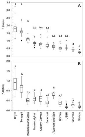
Figure 2: Boxplots showing the hydraulic conductivity (K) values, in cm/s, estimated from 11 empirical formulas for 12 sediment samples in December 2012 (A) and 24 sediment samples in June and July 2013 (B). The letters a, b, c, d, e, f and g, represent significantly different K estimated values (Tukey’s HSD test, P < 0.05), while the signs (+, x and •) are the outliers. Figura 2: Boxplots que muestran los valores de conductividad hidráulica (K), en cm/s, estimados a partir de 11 fórmulas empíricas para 12 muestras de sedimentos en diciembre de 2012 (A) y 24 muestras de sedimentos en junio y julio de 2013 (B). Las letras a, b, c, d, e, f y g, representan valores estimados de K significativamente diferentes (prueba HSD de Tukey, P < 0,05), mientras que los signos (+, x y •) son los valores atípicos.
Discussion
This study clearly evidences that each of the empirical formulas chosen yields different K values. This was not surprising since other authors also find different formulas gave a range of K values for the same sediment by a factor of 10 or even up to ± 20 times (Vukovic and Soro, 1992), and then it becomes critical for the selection of the best appropriate formula to apply for a specific sediment sample.
In Tables 1 and 2, according to the applicability domain of the empirical formulas, 6 samples were not applicable to the Beyer formula because their effective diameter (d10) was greater than 0.6 mm. The Beyer formula is most useful for analysing heterogeneous samples with well-graded grains (Pinder and Celia, 2006), so it is not applicable for our uniformly graded samples. As our samples were not very well sorted, the Krumbein and Monk formula might not be also the most convenient for our studied samples.
For the sand sediments we would expect K to be situated within previously reported limits [i.e., from 0.0001 to 1 cm/s (Freeze and Cherry, 1979)]. Among the formulas we applied, the Beyer and Terzaghi formulas gave the highest K with mean values higher than 1 cm/s while the USBR, Slichter and Harleman formulas gave the lowest K for sand sediments of the Tordera River (Figures 2A and 2B). Similarly, Vukovic and Soro (1992), and Cheng and Chen (2007) reported also underestimation of K when applying the Slichter and USBR formulas. On the other hand, in the case of the Terzaghi formula, Odong (2007) assured that it gives low K values in contrast to our findings, even though this author used the same average sorting coefficient (P) as us. As for the Harleman formula, our study results confirmed the tendency of underestimating K as similarly found by Lu et al. (2012). Moreover, the latter authors highlitghted the Kozeny formula overestimated K in their study but ours reported this formula significantly similar to the formulas of USBR, and Alyamani and §en in December and to those of Harleman, Sauerbrei, and Krumbein and Monk in June and July (Figure 2).
Rosas et al. (2013) while comparing many different empirical formulas highlighted the ones from Hazen and Kozeny-Carman as the most commonly used to estimate K values from grain-size distribution. This is consistent to our results where K values from both formulas were within the range of our first in situ observations with values between 0.20 and 0.75 cm/s calculated by infiltration measurements. However, Carrier (2003) recommended that the Hazen formula should be retired and the Kozeny-Carman formula be adopted because the Hazen formula for predicting the permeability of sand is based only on the effective diameter (d10), whereas the Kozeny-Carman formula (proposed by Kozeny and later modified by Carman) is based on the entire grain-size distribution, the particle shape, and the void ratio (Kozeny, 1927, 1953; Carman, 1937, 1956). As a consequence, the Hazen formula might be less accurate than that of Kozeny-Carman. This agrees with the K values of Odong (2007) confirming that the Kozeny-Carman formula proved to be the best estimator of most samples analysed, and may be the case, even for a wide range of other soil types. In parallel, the results presented in the study of Chapuis and Aubertin (2003) showed that, as a general rule, the Kozeny-Carman formula predicts fairly well the saturated hydraulic conductivity of most soils. The Kozeny-Carman formula, however, estimated some high K values for some samples from December in our study (Figure 2A); and also underestimated a sample in the study of Odong (2007), this was because of that the formula is not appropriate if the particle distribution has a long flat tail in the finer fraction (Carrier, 2003). On the other side, there is a large consensus in the geotechnical literature that the K values of compacted clays (clay liners and covers) cannot be well predicted by the Kozeny-Carman formula (Chapuis and Aubertin, 2003). Despite the adoption of the Kozeny-Carman formula, the classical soil mechanics textbooks maintain that it is approximately valid for sands (Taylor, 1948; Lambe and Whitman, 1969), but it is not valid for clays. However, recently Steiakakis et al. (2012) showed that the Kozeny-Carman formula provides good prediction of the K values of homogenized clayey soils compacted under given compactive effort, despite the consensus set out in the literature.
Altogether, our study results suggest that the Kozeny-Carman formula can be successfully applied to our coarse loose sand sediments because they contained very little content of clay (about 0.7 %, Table 2). Alternatively, respecting to the obtained results, another approach which is likely to be also chosen together with the Kozeny-Carman formula would be that of Sauerbrei (r = 0.93, P < 0.001; ranged from 0.17 to 0.87 cm/s). The latter might be also applicable to the sand samples (Table 1, Figure 2). But, the values from that formula were not as reliable as the Terza-ghi, and Shepherd formulas due to the inconsistent fluctuation of the average estimates at each of the test sites (Lu et al, 2012). When looking at the results from Alyamani and §en formula, K values (0.4-0.9 cm/s) were in the higher limits of K expected for the similar sediments by Freeze and Cherry (1979); and values were poorly correlated with the K values estimated by the Kozeny-Carman formula (r = 0.22, P = 0.202). In addition, the Alyamani and §en formula is particularly very sensitive to the shape of the grading curve and is more accurate for well-graded sample (Odong, 2007) and thus not useful for our uniformly graded samples.
Conclusion
In summary, hydraulic conductivity (K) is correlated with soil properties like pore size and grain-size distribution, and soil texture and this link can be, in part, defined by specific empirical formulas. Most of the empirical formulas use the effective diameter (d10), as a specific aspect of the grain-size distribution that can impact significantly on the permeability of the porous layers. We need to be prudent about the applicability domain of each empirical formula. In the end, although from our data, we suggest using the Kozeny-Car-man formula to calculate K from grain-size distribution; the next step would be measuring K with experimental approaches to check the choice. Interestingly, Song et al. (2009), Lu et al. (2012) and Rosas et al. (2013) showed some correlations between the outcomes from experimental approaches [such as a standard constant head described in Balsillie and Tanner (1995), falling-head standpipe permeameter tests, a permeameter test] with those predicted by the empirical relations but still no new empirical equations have been developed that accurately predict K from these relations yet. After doing so, the more reliable K values we obtain, the more we could understand about the changes in hydrogeochemical processes in the hyporheic zones, since it plays a key relevant role in fluvial ecosystems functioning (Triska et al., 1993; Valett et al.., 1994).

